4.2 Reaction Diffusion

As a third example, let's explore a scenario where a compute shader collaborates with a rendering shader. The compute shader engages in a straightforward simulation known as reaction-diffusion, while the rendering shader is responsible for visualizing the outcomes of this simulated process.

In his groundbreaking 1952 paper, "The Chemical Basis of Morphogenesis", Alan Turing proposed a mathematical model to elucidate the emergence of complex patterns and structures within biological systems, particularly in the realm of embryonic development.

Turing's model explores the interaction of two chemicals undergoing reaction and diffusion processes. This concept, commonly termed the Turing pattern, has become associated with reaction-diffusion systems. Reaction-diffusion equations delineate how concentrations of substances evolve over space and time, influenced by both chemical reactions and substance diffusion. In the realm of pattern formation, Turing's concepts laid the groundwork for comprehending how elementary local interactions could give rise to the development of intricate patterns within biological systems. Despite the seeming simplicity of the reaction-diffusion system, Turing theorized that it underlies the intricate patterns observed in animals, such as zebras and leopards.

In our simulation, we simulate the behavior of two chemicals, A and B. Specifically, two molecules of B catalyze the conversion of one molecule of A into B. Chemical A is introduced into the system at a specified rate, while chemical B exits the system at a distinct rate. This dynamic interplay between the addition of chemical A and the removal of chemical B contributes to the evolving state of the simulation, reflecting the intricate balance and interactions within the simulated reaction-diffusion system.

However, we don't want to model individual molecules. Instead, we divide the entire space into small units, with each unit representing a pixel. For each time step interval, we update the amount of A and B in each pixel, and their concentrations will be visualized using color. The whole process can be described by the following equations:

\begin{aligned} A^\prime &= A + (D_A \nabla^2 A - A B^2 + f(1-A) )\Delta t \\ B^\prime &= B + (D_B \nabla^2 B + A B^2 - (K+f)B)\Delta t \end{aligned}

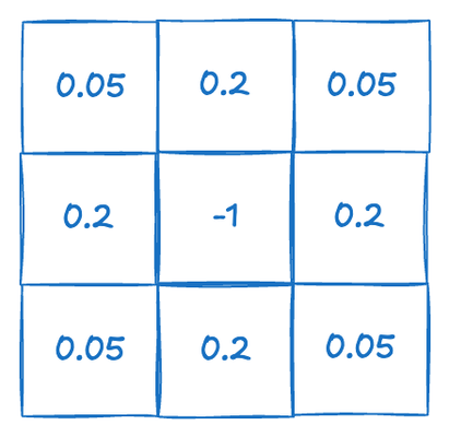
This first equation models the behavior of chemical A. For each unit time \Delta t, the diffused amount is defined by D_A \nabla^2 A, where D_A \nabla^2 is called the Laplacian. The Laplacian is essentially a 3x3 matrix used to calculate a weighted sum of each 3x3 neighborhood. If the center pixel has a higher concentration than its neighbors, we allow more chemical to flow into the neighboring pixels. Conversely, if the neighbors have a higher concentration, the chemical flows from the neighbors into the central pixel.

The Laplacian

The second part of the equation models the chemical reaction. For the reaction to occur, two molecules of B and one molecule of A are required. Since we are modeling the chemicals by their concentration, we can interpret this as the probability of encountering a molecule. This makes sense because the higher the concentration of a chemical, the greater the likelihood of a molecule encounter. Therefore, A B^2 represents the probability of one A molecule encountering two B molecules.

Finally, we add new molecules of A into the system at a rate of f(1-A). This ensures that the concentration of A will not exceed 1.0 because if it does, the rate will become negative to counteract the effect.

Similarly, we remove B molecules at a rate of (K+f)B. Since K + f > f, this ensures that B is removed faster than A is added.

\Delta t is the time interval.

Now let's look at the code. The purpose of this exercise is to demonstrate how a compute shader can work in conjunction with a rendering shader. Two storage textures are involved in the program. Unlike a normal texture, a storage texture can be written to. We use two textures; for each shader invocation, one texture serves as the input, containing the current chemical concentrations. We update the concentrations based on the equations and write the results into the other storage texture. Then we trigger the rendering program for visualization. In consecutive runs, we switch the roles of the two textures. The previous input texture becomes the output and vice versa.

enable chromium_experimental_read_write_storage_texture;

@binding(0) @group(0) var texSrc : texture_storage_2d<rg32float, read>;
@binding(1) @group(0) var texDst : texture_storage_2d<rg32float, write>;
@binding(2) @group(0) var<uniform> drawPos : vec3<f32>;

const imageSize:i32 = 1024;

First, let's define the inputs of the compute shader. In the initial line, we need to explicitly enable the writable storage texture feature, as this feature is still experimental. This is not the only step required to enable this feature; we will also need to request it when we initialize the device, which we will see later.

As previously mentioned, there are two texture maps: one for inputs and one for outputs. Note that the format of the two texture maps is rg32f. Since we have two types of chemicals, we use two channels to represent them. We choose 32f for numerical accuracy.

We also have a drawPos, which defines a position. This position represents the current brush location. Because we want our demo to be interactive, we allow users to draw on the canvas by adding chemical A at the brush's position.

For the image size, we hardcode it to 1024.

@compute @workgroup_size(16, 16)
fn main(@builtin(global_invocation_id) GlobalInvocationID : vec3<u32>) {

      var centerY:i32 = i32(GlobalInvocationID.y);
      var centerX:i32 = i32(GlobalInvocationID.x);

      if (drawPos.z > 0.5) {
          var radius:f32 = sqrt((f32(centerX) - drawPos.x)*(f32(centerX) - drawPos.x) +
          (f32(centerY) - drawPos.y)*(f32(centerY) - drawPos.y));

          if (radius < 5.0) {
              textureStore(texDst, vec2i(GlobalInvocationID.xy), vec4<f32>(0.0,1.0,0.0,0.0));
              return;
          }
      }

}

Next, we create a compute kernel function. Notice that we are using a 2D workgroup of size 16x16. The 2D workgroup is suitable because our problem involves calculating pixel values for a 2D texture map. Although 16x16 may seem small compared to the texture map size of 1024, this size is the maximum workgroup size we can request. This is due to the maxComputeInvocationsPerWorkgroup limitation, which is 256 (the maximum value of the product of the workgroup dimensions for a compute stage).

Next, we handle the brush input. If the user is actively drawing (determined by drawPos.z > 0.5), we compute the distance between the current pixel (centerX, centerY) and drawPos.xy. If this distance is less than 5.0, we set the texture color to (0.0, 1.0), indicating that the pixel is fully concentrated with molecule B.

for(var y = -1; y<= 1;y++) {
    var accessY:i32 = centerY + y;
    if (accessY < 0) {
        accessY = imageSize-1;
    } else if (accessY >= imageSize) {
        accessY = 0;
    }

    for(var x = -1; x<=1;x++) {
        var accessX:i32 =centerX+ x;

        if (accessX < 0) {
            accessX = imageSize-1;
        } else if (accessX >= imageSize) {
            accessX = 0;
        }
        var rate = -1.0;
        if (x==0 && y == 0) {
            rate = -1.0;
        } else if (x ==0 || y==0) {
            rate = 0.2;
        } else {
            rate = 0.05;
        }
        data += textureLoad(texSrc, vec2i(accessX, accessY)).rg * rate;
    }
}

Here, we loop through the 3x3 neighborhood surrounding the current pixel. We ensure that if the indices fall outside the image boundaries, they wrap around to the opposite edge of the image.

var rate = -1.0;
if (x==0 && y == 0) {
    rate = -1.0;
} else if (x ==0 || y==0) {
    rate = 0.2;
} else {
    rate = 0.05;
}
data += textureLoad(texSrc, vec2i(accessX, accessY)).rg * rate;

We then calculate the change in concentration due to diffusion. The rate variable determines how much influence each neighboring pixel has based on its distance from the center pixel.

const f:f32 = 0.055;
const k:f32 = 0.062;
data = vec2<f32>(data.x- original.x*original.y*original.y
    + f * (1.0 - original.x),
     data.y*0.5 + original.x*original.y*original.y - (k+f) * original.y) + original;
textureStore(texDst, vec2i(GlobalInvocationID.xy), vec4<f32>(data,0.0,0.0));

Finally, we compute the concentration changes due to the reaction and update the system accordingly. The result is then written to the output texture map.

For visualization, the rendering shader functions similarly to a basic texture mapping shader. It displays the results from the compute shader by mapping them onto a quad. Note that for the rendering shader, the texture used does not need to be a storage texture; a standard texture map type suffices.

Now let's look at pipeline configuration.

const feature = "chromium-experimental-read-write-storage-texture";
const adapter = await navigator.gpu.requestAdapter();
console.log(adapter);
if (!adapter.features.has(feature)) {
    showWarning("This sample requires a chrome experimental feature. Please restart chrome with the --enable-dawn-features=allow_unsafe_apis flag.");
    throw new Error("Read-write storage texture support is not available");
}
const device = await adapter.requestDevice({
    requiredFeatures: [feature],
});

First, as previously mentioned, it's essential to request support for the storage texture feature when creating the GPU device.

Next, configure the uniforms for the compute stage as follows:

const context = configContext(device, canvas)

// create shaders
let shaderModule = shaderModuleFromCode(device, 'shader');

let uniformBindGroupLayoutCompute = device.createBindGroupLayout({
    entries: [
        {
            binding: 0,
            visibility: GPUShaderStage.COMPUTE,
            storageTexture: {
                access: "read-only",
                format: "rg32float",
            }
        },
        {
            binding: 1,
            visibility: GPUShaderStage.COMPUTE,
            storageTexture: {
                access: "write-only",
                format: "rg32float",
            }
        },
        {
            binding: 2,
            visibility: GPUShaderStage.COMPUTE,
            buffer: {}
        }
    ]
});

This configuration is akin to previous setups, with particular attention paid to the storage texture’s specification. The input texture is designated as read-only, while the output texture is set to write-only. The format used is rg32float, ensuring sufficient precision for the chemical concentrations.

Next, we proceed to initialize the input texture. This step is crucial as it assigns initial chemical concentrations to the texture. By doing this, the simulation can generate patterns autonomously, even in the absence of user interaction. This setup allows the system to develop and evolve patterns based on predefined initial conditions, facilitating a meaningful demonstration of the reaction-diffusion process.

const srcTextureDesc = {
    size: [1024, 1024, 1],
    dimension: '2d',
    format: "rg32float",
    usage: GPUTextureUsage.COPY_DST | GPUTextureUsage.STORAGE_BINDING | GPUTextureUsage.TEXTURE_BINDING
};

let textureValues = [];

for (let y = 0; y < 1024; ++y) {
    for (let x = 0; x < 1024; ++x) {
        if (x > 302 && x < 532 && y >= 302 && y < 532) {
            textureValues.push(0.0);
            textureValues.push(1.0);
        }
        else {
            textureValues.push(1.0);
            textureValues.push(0.0);
        }
    }
}

let srcTexture = device.createTexture(srcTextureDesc);

device.queue.writeTexture({ texture: srcTexture }, new Float32Array(textureValues), {
    offset: 0,
    bytesPerRow: 1024 * 8,
    rowsPerImage: 1024
}, { width: 1024, height: 1024 });
await device.queue.onSubmittedWorkDone();

To initialize the texture map, we define a rectangular area [302, 532, 302, 532] within which chemical B is assigned, and outside this rectangle, chemical A is used. This setup is straightforward and ensures that the initial conditions for the simulation are well-defined. The resulting data is then loaded into the input texture.

const dstTextureDesc = {
    size: [1024, 1024, 1],
    dimension: '2d',
    format: "rg32float",
    usage: GPUTextureUsage.COPY_SRC | GPUTextureUsage.STORAGE_BINDING | GPUTextureUsage.TEXTURE_BINDING
};

let dstTexture = device.createTexture(dstTextureDesc);

let drawPosUniformBuffer = createGPUBuffer(device, drawPos, GPUBufferUsage.UNIFORM | GPUBufferUsage.COPY_DST);

Next, we create the output texture, which doesn’t require any initialization. To manage the alternating roles of the input and output textures between consecutive invocations, we set up two uniform bind groups:

let uniformBindGroupCompute0 = device.createBindGroup({
    layout: uniformBindGroupLayoutCompute,
    entries: [
        {
            binding: 0,
            resource: srcTexture.createView()
        },
        {
            binding: 1,
            resource: dstTexture.createView()
        },
        {
            binding: 2,
            resource: {
                buffer: drawPosUniformBuffer
            }
        }
    ]
});

let uniformBindGroupCompute1 = device.createBindGroup({
    layout: uniformBindGroupLayoutCompute,
    entries: [
        {
            binding: 0,
            resource: dstTexture.createView()
        },
        {
            binding: 1,
            resource: srcTexture.createView()
        },
        {
            binding: 2,
            resource: {
                buffer: drawPosUniformBuffer
            }
        }
    ]
});

Following this, we need to set up the compute shader pipeline. As this process mirrors previous examples, the code is omitted here. Once the compute shader is configured, we proceed to configure the bind group layout for the rendering shader:

const sampler = device.createSampler({
    addressModeU: "clamp-to-edge",
    addressModeV: "clamp-to-edge",
    addressModeW: "clamp-to-edge",
    magFilter: "nearest",
    minFilter: "nearest",
    mipmapFilter: "nearest"
});

let uniformBindGroupLayoutRender = device.createBindGroupLayout({
    entries: [
        {
            binding: 0,
            visibility: GPUShaderStage.FRAGMENT,
            texture: {
                sampleType: "unfilterable-float",
            }
        },
        {
            binding: 1,
            visibility: GPUShaderStage.FRAGMENT,
            sampler: {
                type: "non-filtering",
            }
        }
    ]
});

Unless the feature "float32-filterable" is enabled, the texture format rg32float can only use unfilterable-float for its sampleType. Consequently, the sampler must employ "nearest" for filtering and be of type "non-filtering." Filtering in computer graphics involves interpolating the values defined on the texture map to determine what is read in a shader program. During texture mapping, a texture lookup determines where each pixel center falls on the texture. On texture-mapped polygonal surfaces, typical in 3D games and movies, each pixel (or subordinate pixel sample) corresponds to some triangles and a set of barycentric coordinates, which define its position within the texture. Since the textured surface may be at an arbitrary distance and orientation relative to the viewer, one pixel does not usually align directly with one texel. Filtering is necessary to determine the best color for the pixel and to avoid artifacts such as blockiness, jaggies, or shimmering.

The relationship between a pixel and the texel(s) it represents on the screen varies based on the textured surface's position relative to the viewer. For example, when a square texture is mapped onto a square surface, and the viewing distance makes one screen pixel exactly the same size as one texel, no filtering is required. However, if the texels are larger than the screen pixels (texture magnification), or if each texel is smaller than a pixel (texture minification), appropriate filtering is needed. Graphics APIs like OpenGL allow programmers to set different filters for magnification and minification.

Even when pixels and texels are the same size, a pixel may not align perfectly with a texel and may cover parts of up to four neighboring texels. Therefore, filtering is still necessary.

In our demo, we will bypass the extra requirement of enabling "float32-filterable" by reading values directly from the texture map without interpolation.

For bind groups, we need to create two separate groups to alternate between the two texture maps:

let uniformBindGroupRender0 = device.createBindGroup({
    layout: uniformBindGroupLayoutRender,
    entries: [
        {
            binding: 0,
            resource: dstTexture.createView()
        },
        {
            binding: 1,
            resource: sampler
        }
    ]
});

let uniformBindGroupRender1 = device.createBindGroup({
    layout: uniformBindGroupLayoutRender,
    entries: [
        {
            binding: 0,
            resource: srcTexture.createView()
        },
        {
            binding: 1,
            resource: sampler
        }
    ]
});

The remaining code for setting up the rendering pipeline is similar to previous examples, so I'll omit the details. Now, let's address implementing brush drawing. The pattern produced by the reaction-diffusion process is sensitive to the initial chemical concentration, so we need to allow users to alter this concentration to modify the pattern. To achieve this, we add brush drawing capabilities.

Here’s how we handle mouse input for brush drawing:

let prevX = 0.0;
let prevY = 0.0;
let isDragging = false;

canvas.onmousedown = (event) => {
    var rect = canvas.getBoundingClientRect();
    const x = event.clientX - rect.left;
    const y = event.clientY - rect.top;


    isDragging = true;

}

canvas.onmousemove = (event) => {
    if (isDragging != 0) {
        var rect = canvas.getBoundingClientRect();
        const x = event.clientX - rect.left;
        const y = event.clientY - rect.top;
        drawPos.set([x, y, 1.0], 0);
    }
}

canvas.onmouseup = (event) => {
    isDragging = 0;
    drawPos.set([0.0, 0.0, 0.0], 0);
}

The implementation is straightforward: we update the uniform drawPos to (x, y, 1.0) when the user is drawing, and set it to (0.0, 0.0, 0.0) when not. In the shader code, the third component of this vector (drawPos.z > 0.5) is used to check if the brush is actively touching the canvas.

const passEncoder = commandEncoder.beginComputePass(
    {}
);
passEncoder.setPipeline(computePipeline);
if (frame % 2 == 0) {
    passEncoder.setBindGroup(0, uniformBindGroupCompute0);
}
else {
    passEncoder.setBindGroup(0, uniformBindGroupCompute1);
}
passEncoder.dispatchWorkgroups(64, 64);
passEncoder.end();

device.queue.submit([commandEncoder.finish()]);

const commandEncoder2 = device.createCommandEncoder();

const passEncoder2 = commandEncoder2.beginRenderPass(renderPassDesc);
passEncoder2.setViewport(0, 0, canvas.width, canvas.height, 0, 1);
passEncoder2.setPipeline(renderPipeline);
if (frame % 2 == 0) {
    passEncoder2.setBindGroup(0, uniformBindGroupRender0);
}
else {
    passEncoder2.setBindGroup(0, uniformBindGroupRender1);
}
passEncoder2.setVertexBuffer(0, positionBuffer);
passEncoder2.draw(4, 1);
passEncoder2.end();

The rendering process consists of two distinct passes. The first pass performs the compute operations and updates the output texture map, while the second pass renders the updated texture map onto the screen. Note that the compute shader uses a workgroup size of 16x16, and we dispatch the workgroups in a 2D formation of 64x64. This is because 64x16 equals 1024, which matches the size of our textures.

This completes one frame of rendering. For the next frame, we will switch the roles of the input and output textures: the output texture will become the input, and the input texture will become the output.

Show 3 Steps of Diffusion