1.15 Understanding Normals

In this tutorial, we explore into the concept of normals, a crucial element in all aspects of computer graphics. Normals are extensively used in lighting calculations, as lighting effects in computer graphics depend on how light interacts with a surface's material. The direction from which light strikes a surface can significantly alter its appearance, making it essential to determine where a surface is facing. This directional aspect is referred to as the normal direction.

Flat vs. Smooth Normals Visualized in 2D

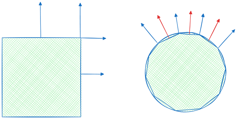
The concept of a surface's facing direction is a simplified description. In reality, how normals change on a surface and where they should be defined can vary depending on the application. In the simplest scenario, when rendering flat surfaces with sharp creases or features, we can attach one normal to each face, allowing normals to change abruptly at these features. An edge or vertex joining multiple faces will likely have multiple normals, one for each adjacent face, reflecting the discontinuity of surface smoothness.

Vertex Normals Can Be Interpolated on a Triangle, Generating Smooth Normal Transitions

In other scenarios, we might prefer a smooth surface where normals don't change suddenly. In this case, normals can be defined on vertices instead, as an average of nearby surface normals. These vertex-defined normals will be interpolated during the rasterization stage, generating smooth normal transitions across triangles and resulting in smoother rendering.

For more complex cases, such as modeling microstructures like rough walls or wrinkled surfaces, both per-face and per-vertex normals may lack sufficient resolution. In these situations, we can store normals in a texture map, allowing a single triangle to have numerous normals sampled from the texture.

Normals can be calculated based on geometry or loaded from a file. Most 3D model files contain not only vertex positions but also normals. In this tutorial, we extend our loading logic to include normals.

for (let f of obj.result.models[0].faces) {
    let points = [];
    let facet_indices = [];
    for (let v of f.vertices) {
        const index = v.vertexIndex - 1;
        indices.push(index);

        const vertex = glMatrix.vec3.fromValues(positions[index * 3], positions[index * 3 + 1], positions[index * 3 + 2]);

        minX = Math.min(positions[index * 3], minX);
        maxX = Math.max(positions[index * 3], maxX);

        minY = Math.min(positions[index * 3 + 1], minY);
        maxY = Math.max(positions[index * 3 + 1], maxY);

        minZ = Math.min(positions[index * 3 + 2], minZ);
        maxZ = Math.max(positions[index * 3 + 2], maxZ);
        points.push(vertex);
        facet_indices.push(index);
    }

    const v1 = glMatrix.vec3.subtract(glMatrix.vec3.create(), points[1], points[0]);
    const v2 = glMatrix.vec3.subtract(glMatrix.vec3.create(), points[2], points[0]);
    const cross = glMatrix.vec3.cross(glMatrix.vec3.create(), v1, v2);
    const normal = glMatrix.vec3.normalize(glMatrix.vec3.create(), cross);

    for (let i of facet_indices) {
        normals[i * 3] += normal[0];
        normals[i * 3 + 1] += normal[1];
        normals[i * 3 + 2] += normal[2];
    }
}
let normalBuffer = createGPUBuffer(device, normals, GPUBufferUsage.VERTEX);

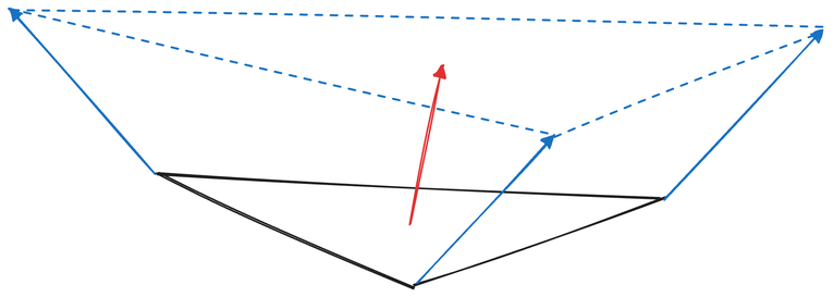
We calculate normals as the cross product of two of a triangle edges.

@group(0) @binding(0)
var<uniform> modelView: mat4x4<f32>;
@group(0) @binding(1)
var<uniform> projection: mat4x4<f32>;
@group(0) @binding(2)
var<uniform> normal: mat4x4<f32>;

In the shader code, we introduce a new uniform called normal transformation, which is a distinct transformation matrix for normals. Although this transformation matrix is derived from the same modelview matrix applied to geometry, we cannot simply use the modelview matrix for normal transformation.

2D Illustration of a Normal Under Non-Uniform Scaling

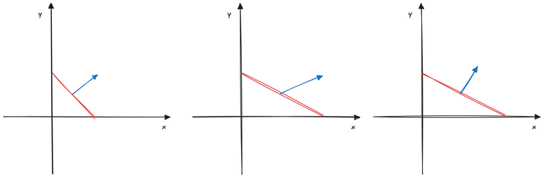
Understanding the reason for this separate transformation is a key takeaway of this tutorial. Let's explain using a 2D illustration. Imagine we have a line and its normal, and we apply a transformation to it. As long as the transformation involves only translation, rotation, and uniform scaling, the normal, under the same transformation, should remain perpendicular to the transformed line. However, this does not hold true if non-uniform scaling is involved. For example, if we stretch the line along the x-axis only, the new normal under the same stretch is no longer perpendicular to the line. Consequently, we need to find a different transformation for the normals that ensures they remain perpendicular to the surfaces after transformation.

To understand this mathematically, let's consider two vectors v and n, where v is the tangent vector of the original surface and n is the original surface normal. They exhibit the following relationship due to their perpendicularity:

v \times n^\intercal = 0

Let M be the transformation matrix. We know that MM^{-1} = \mathbb{I}, where \mathbb{I} is the identity matrix. If we incorporate this into the equation above, we obtain:

\begin{aligned} v \times n^\intercal &= 0 \\ v \times M \times M^{-1} \times n^\intercal &= 0 \\ v \times M \times (n \times M^{-1\intercal})^\intercal &= 0 \end{aligned}

Since v \times M represents the transformed tangent vector, let's denote it as v^\prime. We know that v^\prime \times (n^\prime)^\intercal = 0, where n^\prime is the transformed normal. Therefore, we can deduce:

n^\prime = n \times M^{-1\intercal}

Therefore, M^{-1\intercal} is the normal transformation matrix we seek, which is the transpose of the inverse of the modelview matrix. Having derived the appropriate normal transformation matrix, let's examine the corresponding shader code:

struct VertexOutput {
    @builtin(position) clip_position: vec4<f32>,
    @location(0) normal: vec3<f32>
};

@vertex
fn vs_main(
    @location(0) inPos: vec3<f32>,
    @location(1) inNormal: vec3<f32>
) -> VertexOutput {
    var out: VertexOutput;
    out.clip_position = projection * modelView * vec4<f32>(inPos, 1.0);
    out.normal = normalize(normal * vec4<f32>(inNormal, 0.0)).xyz;
    return out;
}

In the vertex stage entry point, we introduce a new vertex attribute at @location(1) called inNormal. This attribute is a vector of three floating-point values representing the surface normal. We apply the normal transformation to this input, and the resulting transformed normal is typically passed to the fragment shader, where lighting calculations are performed.

@fragment
fn fs_main(in: VertexOutput,  @builtin(front_facing) face: bool) -> @location(0) vec4<f32> {
    if (face) {
        var normal:vec3<f32> = normalize(in.normal);
        return vec4<f32>(normal ,1.0);
    }
    else {
        return vec4<f32>(0.0, 1.0, 0.0 ,1.0);
    }
}

Normals are typically utilized in rendering algorithms within the fragment shader. However, since we haven't yet discussed lighting or other complex rendering algorithms that involve normals, we'll simply visualize them by rendering them as colors for this tutorial. We first normalize the normal vectors because the interpolation process during rasterization can affect their length. By definition, normals are always unit vectors as they represent directions. This color-based visualization helps us understand the distribution of normals across the surface.

const normalAttribDesc = {
    shaderLocation: 1, // @location(1)
    offset: 0,
    format: 'float32x3'
};

const normalBufferLayoutDesc = {
    attributes: [normalAttribDesc],
    arrayStride: 4 * 3, // sizeof(float) * 3
    stepMode: 'vertex'
};

Moving on to the JavaScript code, we introduce a normal attribute descriptor. This descriptor is similar to the position attribute descriptor, but it specifies shaderLocation as 1 to correspond with the @location(1) we defined for normals in the shader code.

const pipelineDesc = {
    layout,
    vertex: {
        module: shaderModule,
        entryPoint: 'vs_main',
        buffers: [positionBufferLayoutDesc, normalBufferLayoutDesc]
    },
    fragment: {
        module: shaderModule,
        entryPoint: 'fs_main',
        targets: [colorState]
    },
    primitive: {
        topology: 'triangle-list',
        frontFace: 'ccw',
        cullMode: 'none'
    },
    depthStencil: {
        depthWriteEnabled: true,
        depthCompare: 'less',
        format: 'depth24plus-stencil8'
    }
};

When defining the pipeline descriptor, we must provide both the position and normal buffers as vertex buffers. Consequently, during the rendering process, two vertex buffers need to be set.

Teapot Colored With Normals

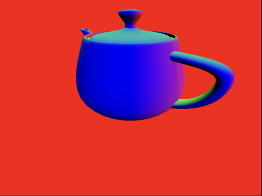
Now, let's proceed to render the teapot. Upon visualization, you'll observe that the teapot's surface exhibits a vibrant spectrum of colors. These colors correspond to the normal directions at each point on the surface. Since we've defined our normals at the vertex level, and the GPU handles the interpolation from the vertex buffer to the fragment shader, the color transition across the teapot's surface appears remarkably smooth. There are no discernible triangles or sharp edges, demonstrating the effectiveness of this technique. This smooth transition of normals is crucial for achieving realistic and seamless lighting effects in more complex rendering scenarios.