1.1 Drawing a Triangle

Our first tutorial is a bit boring as we weren't drawing anything. In this tutorial, we will draw a single triangle.

In the realm of 3D rendering, triangles serve as the most foundational elements to draw. They stand as the pixels of a 3D world, making them an ideal starting point for our first tutorial. Here, we will learn how to draw a single triangle. Our journey will involve crafting a straightforward shader to define pixel colors within a triangle, along with understanding how to establish a graphics pipeline that takes this triangle and renders it on the screen using the shader. Just like the "Hello World" program in traditional programming, drawing a triangle serves as the equivalent introduction to any graphics API.

In our previous example, we didn't create any shader. As mentioned before, a shader program is a program executed on the GPU. In general, there are three main types of shader programs: vertex shaders, fragment shaders, and compute shaders. While compute shaders are used for general-purpose computations, vertex and fragment shaders are specifically related to rendering. The vertex shader processes each vertex of our geometry, determining its final position on the screen. The fragment shader then determines the color of each pixel within the shapes defined by these vertices. Together, these shaders work to convert geometry primitives, such as points or triangles, into the pixels you see on your screen.

<script id="shader" type="wgsl">
...
</script>

Now that we understand the role of shaders, let's add them to our project. First, we'll create another script tag in our HTML to hold the shader code. This time, we'll set its type to wgsl, standing for WebGPU shader language. In addition to the type, we also need to give it an id of shader, because we'll need to read its content later. It's worth noting that it's not required to put shader code in a script tag. You can choose to assign your shader code to a JavaScript string, or you could write them into external files and fetch them into your code.

struct VertexOutput {
    @builtin(position) clip_position: vec4<f32>,
};

@vertex
fn vs_main(
    @builtin(vertex_index) in_vertex_index: u32,
) -> VertexOutput {
    var out: VertexOutput;
    let x = f32(1 - i32(in_vertex_index)) * 0.5;
    let y = f32(i32(in_vertex_index & 1u) * 2 - 1) * 0.5;
    out.clip_position = vec4<f32>(x, y, 0.0, 1.0);
    return out;
}

@fragment
fn fs_main(in: VertexOutput) -> @location(0) vec4<f32> {
    return vec4<f32>(0.3, 0.2, 0.1, 1.0);
}

Our first shader renders a triangle in a solid color. Despite sounding simple, the code may seem complex at first glance. Let's dissect it to understand its components better.

Shader programs define the behavior of a GPU pipeline. A GPU pipeline works like a small factory, containing a series of stages or workshops. A typical GPU pipeline consists of two main stages:

1. Vertex Stage: Processes geometry data and generates canvas-aligned geometries.

2. Fragment Stage: After the GPU converts the output from the vertex stage into fragments, the fragment shader assign them a color.

In our shader code, there are two entry functions:

• vs_main: Represents the vertex stage, annotated by @vertex

• fs_main: Represents the fragment stage, annotated by @fragment

While the input to the vs_main function @builtin(vertex_index) in_vertex_index: u32 looks similar to function parameters in languages like C, it's different. Here, in_vertex_index is the variable name, and u32 is the type (a 32-bit unsigned integer). The @builtin(vertex_index) is a special decorator that requires explanation.

In WGSL, shader inputs aren't truly function parameters. Instead, imagine a predefined form with several fields, each with a label. @builtin(vertex_index) is one such label. For a pipeline stage's inputs, we can't freely feed any data; we must select fields from this predefined set. In this case, @builtin(vertex_index) is the actual parameter name, and in_vertex_index is just an alias we've given it.

The @builtin decorator indicates a group of predefined fields. We'll encounter other decorators like @location, which we'll discuss later to understand their differences.

Shader stage outputs follow a similar principle. We can't output arbitrary data; instead, we populate a few predefined fields. In our example, we're outputting a struct VertexOutput, which appears custom-defined. However, it contains a single predefined field @builtin(position), where we'll write our result.

The Screen Space Coordinate System.

The content of the vertex shader may seem puzzling at first. Before we delve into it, let me explain the primary goal of a vertex shader. A vertex shader receives geometries as individual vertices. At this stage, we lack geometry connectivity information, meaning we don't know which vertices connect to form triangles. This information is not available to us. We process individual vertices with the aim of converting their positions to align with the canvas.

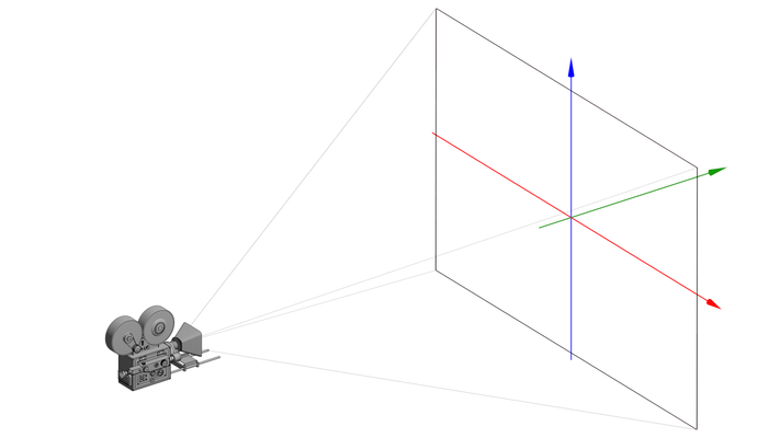
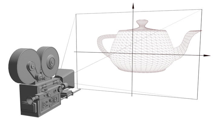
Without this conversion, the vertices wouldn't be visible correctly. Vertex positions, as received by a vertex shader, are typically defined in their own coordinate system. To display them on the canvas, we must unify the coordinate systems used by the input vertices into the canvas' coordinate system. Additionally, vertices can exist in 3D space, while the canvas is always 2D. In computer graphics, the process of transforming 3D coordinates into 2D is called projection.

Now, let's examine the coordinate system of the canvas. This system is usually referred to as the screen space or clip space. Although in WebGPU we typically render to a canvas rather than directly to a screen, the term "screen space coordinate system" is inherited from other native 3D APIs.

The screen space coordinate system has its origin at the center, with both x and y coordinates confined within the [-1, 1] range. This coordinate system remains constant regardless of your screen or canvas size.

Recall from the previous tutorial that we can define a viewport, but this doesn't affect the coordinate system. This may seem counter-intuitive. The screen space coordinate system remains unchanged regardless of your viewport definition. A vertex is visible as long as its coordinates fall within the [-1, 1] range. The rendering pipeline automatically stretches the screen space coordinate system to match your defined viewport. For instance, if you have a viewport of 640x480, even though the aspect ratio is 4:3, the canvas coordinate system still spans [-1, 1] for both x and y. If you draw a vertex at location (1, 1), it will appear at the upper right corner. However, when presented on the canvas, the location (1, 1) will be stretched to (640, 0).

The Visible Area Remains Constant Regardless of Screen Size or Aspect Ratio.

In the code above, our inputs are vertex indices rather than vertex positions. Since a triangle has three vertices, the indices are 0, 1, and 2. Without vertex positions as input, we generate their positions based on these indices, instead of performing vertex position transformation. Our goal is to generate a unique position for each index while ensuring that the position falls within the [-1, 1] range, making the entire triangle visible. If we substitute 0, 1, 2 for vertex_index, we'll get the positions (0.5, -0.5), (0, 0.5), and (-0.5, -0.5) respectively.

let x = f32(1 - i32(in_vertex_index)) * 0.5;
let y = f32(i32(in_vertex_index & 1u) * 2 - 1) * 0.5;

A clip location (a position in the clip space) is represented by a 4-float vector, not just 2. For our 2D triangle in screen space, the third component is always zero. The last value is set to 1.0. We'll delve into the details of the last two values when we explore camera and matrix transformations later.

As mentioned earlier, the outputs of the vertex stage undergo rasterization. This process generates fragments with interpolated vertex values. In our simple example, the only interpolated value is the vertex position.

The fragment shader's output is defined by another predefined field called @location(0). Each location can store up to 16 bytes of data, equivalent to four 32-bit floats. The total number of available locations is determined by the specific WebGPU implementation.

To understand the distinction between locations and builtins, we can consider locations as unstructured custom data. They have no labels other than an index. This concept parallels the HTTP protocol, where we have a structured message header (akin to builtins) followed by a body or payload (similar to locations) that can contain arbitrary data. If you're familiar with decoding binary files, it's comparable to having a structured header with metadata, followed by a chunk of data as the payload. In our context, builtins and locations share this conceptual structure.

Our fragment shader in this example is straightforward: it simply outputs a solid color to @location(0).

let code = document.getElementById('shader').innerText;
const shaderDesc = { code: code };
let shaderModule = device.createShaderModule(shaderDesc);

Writing the shader code is just one part of rendering a simple triangle. Let's now examine how to modify the pipeline to incorporate this shader code. The process involves several steps:

1. We retrieve the shader code string from our first script tag. This is where the tag's id='shader' attribute becomes crucial.

2. We construct a shader description object that includes the source code.

3. We create a shader module by providing the shader description to the WebGPU API.

It's worth noting that we haven't implemented error handling in this example. If a compilation error occurs, we'll end up with an invalid shader module. In such cases, the browser's console messages can be extremely helpful for debugging.

Typically, shader code is defined by developers during the development stage, and it's likely that all shader issues will be resolved before the code is deployed. For this reason, we've omitted error handling in this basic example. However, in a production environment, implementing robust error checking would be advisable.

const pipelineLayoutDesc = { bindGroupLayouts: [] };
const layout = device.createPipelineLayout(pipelineLayoutDesc);

Next, we define the pipeline layout. But what exactly is a pipeline layout? It refers to the structure of constants we intend to provide to the pipeline. Each layout represents a group of constants we want to feed into the pipeline.

A pipeline can have multiple groups of constants, which is why bindGroupLayouts is defined as a list. These constants maintain their values throughout the execution of the pipeline.

In our current example, we're not providing any constants at all. Consequently, our pipeline layout is empty.

const colorState = {
    format: 'bgra8unorm'
};

The next step in our pipeline configuration is to specify the output pixel format. In this case, we're using bgra8unorm. This format defines how we'll populate our rendering target. To elaborate, bgra8unorm stands for:

• 'b', 'g', 'r', 'a': Blue, Green, Red, Alpha channels

• '8': Each channel uses 8 bits

• 'unorm': Values are unsigned and normalized (ranging from 0 to 1)

const pipelineDesc = {
    layout,
    vertex: {
        module: shaderModule,
        entryPoint: 'vs_main',
        buffers: []
    },
    fragment: {
        module: shaderModule,
        entryPoint: 'fs_main',
        targets: [colorState]
    },
    primitive: {
        topology: 'triangle-list',
        frontFace: 'ccw',
        cullMode: 'back'
    }
};

pipeline = device.createRenderPipeline(pipelineDesc);

Having assembled all necessary components, we can now create the pipeline. A GPU pipeline, analogous to a real factory pipeline, consists of inputs, a series of processing stages, and final outputs. In this analogy, layout and primitive describe the input data formats. As previously mentioned, layout refers to the constants, while primitive specifies how the geometry primitives should be provided.

Typically, the actual input data is supplied through buffers. These buffers normally contain vertex data, including vertex positions and other attributes such as vertex colors and texture coordinates. However, in our current example, we don't use any buffers. Instead of feeding vertex positions directly, we derive them in the vertex shader stage from vertex indices. These indices are automatically provided by the GPU pipeline to the vertex shader.

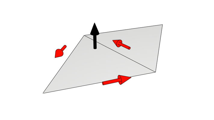
Typically, we provide input geometry as a list of vertices without explicit connectivity information, rather than as complete 3D graphic elements like triangles. The pipeline reconstructs triangles from these vertices based on the topology field. For instance, if the topology is set to triangle-list, it indicates that the vertex list represents triangle vertices in either counter-clockwise or clockwise order. Each triangle has a front side and a back side, with the vertex order defining the direction of the triangle's front face frontFace: 'ccw'.

The cullMode parameter determines whether we want to eliminate the rendering of a particular side of the triangle. Setting it to back means we choose not to render the back side of triangles. In most cases, the back sides of triangles shouldn't be rendered, and omitting them can save computational resources.

Using a triangle list topology is the most straightforward way of representing triangles, but it's not always the most efficient method. As illustrated in the following diagram, when we want to render a strip formed by connected triangles, many of its vertices are shared by more than one triangle.

Two Triangles Form a Triangle Strip. In a Right-Handed System, Positive Vertex Order Is Counterclockwise Around the Triangle Normal

In such cases, we want to reuse vertex positions for multiple triangles, rather than redundantly sending the same position multiple times for different triangles. This is where a triangle-strip topology becomes a better choice. It allows us to define a series of connected triangles more efficiently, reducing data redundancy and potentially improving rendering performance. We will explore other topology types in future chapters.

commandEncoder = device.createCommandEncoder();

passEncoder = commandEncoder.beginRenderPass(renderPassDesc);
passEncoder.setViewport(0, 0, canvas.width, canvas.height, 0, 1);
passEncoder.setPipeline(pipeline);
passEncoder.draw(3, 1);
passEncoder.end();

device.queue.submit([commandEncoder.finish()]);

With the pipeline defined, we need to create the colorAttachment, which is similar to what we covered in the first tutorial, so I'll omit the details here. After that, the final step is command creation and submission. This process is nearly identical to what we've done before, with the key differences being the use of our newly created pipeline and the invocation of the draw() function.

The draw() function triggers the rendering process. The first parameter specifies the number of vertices we want to render, and the second parameter indicates the instance count. Since we are rendering a single triangle, the total number of vertices is 3. The vertex indices are automatically generated for the vertex shader.

The instance count determines how many times we want to duplicate the triangle. This technique can speed up rendering when we need to render a large number of identical geometries, such as grass or leaves in a video game. In this example, we specify a single instance because we only need to draw one triangle.