1.18 Mipmapping and Anisotropic Filtering

Sampling issues can occur in various aspects of rendering. In our previous tutorial, we discussed sampling problems related to low screen resolution. However, these issues can also arise during texture map sampling. Recall that in the texture tutorial, we used the textureSample function to sample colors from a texture map. When a texture map is distant from the camera, its projected size on the screen plane can become very small. If the projected size is significantly smaller than the fragment size, texture sampling issues may occur. This can be illustrated as follows:

Insufficient Texture Sampling Rate Results in Artifacts

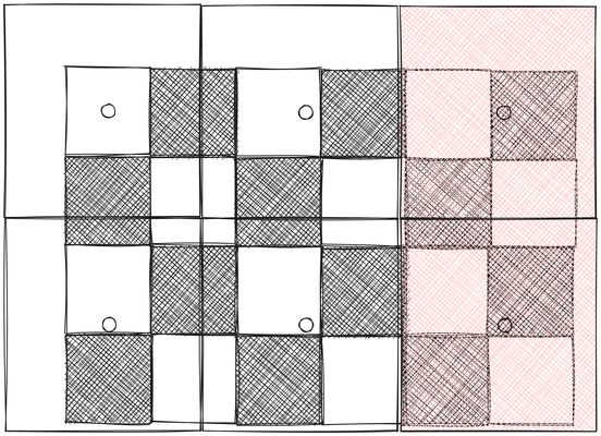
In the above image, we attempt to render a checkerboard, where the larger squares represent fragments. We use the fragment center as the texture coordinates to sample from the checkerboard texture. In this example, only the two rightmost fragments are black, while the rest are white.

This situation is similar to the rasterization issue we encountered in the MSAA tutorial. All these fragments overlap with both white and black checkers. Ideally, when viewed from a distance, they should appear gray rather than strictly black or white.

While using multiple samples per fragment can improve rendering results, it is computationally expensive. Unlike dynamic rendering results, texture maps are static. For a static texture map, there's no need for runtime supersampling. Instead, we can perform this process offline, cache the sampled colors, and read the values during runtime.

In the MSAA tutorial, we used extra samples and calculated the average color as the final color. An alternative method involves downsizing the texture map to smaller sizes. This process also involves averaging pixels, and the downsized texture map acts as a cache for the sampled colors. This method is known as filtering.

It's a misconception that a texture map is simply an image. In fact, a texture map can have multiple levels. In this tutorial, we'll discuss mipmapping, a sampling solution that uses a pyramid of images at different sizes.

Each level typically contains the same image at different resolutions, with level 0 being the original resolution. At level 1, we quarter the original image, and so on until the entire image is downsized to a single pixel representing the average color of the original texture map. We refer to this as the levels of detail.

In the above image, we showed a situation where the texture map is parallel to the screen plane. However, this is rarely the case in practice. We often view textured polygons at an angle. Consequently, there is no single ideal sample rate for an entire textured polygon. Instead, the optimal sample rate must be determined on a per-fragment basis.

To illustrate this concept with actual code, let's examine the same shader we encountered when introducing texture mapping. However, instead of using the baboon texture map, we'll use a checkerboard to make the issue more apparent.

Sampling Artifacts Without Mipmapping

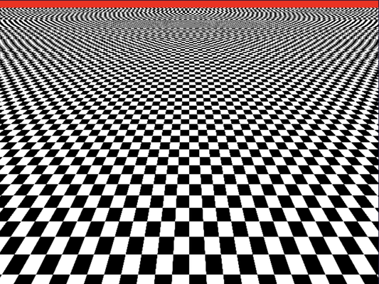
With this naive implementation, the results are clearly visible. On the near side of the checkerboard, we can distinctly see the checkerboard pattern. However, as we look towards the far side, the pattern begins to distort into stripes, no longer resembling a checkerboard. This distortion occurs because we're not sampling the texture map frequently enough.

When sampling fragments, if we happen to consistently fall on black areas, we end up retrieving predominantly black colors from the texture map. The result is a black stripe instead of alternating black and white colors. Similarly, if we consistently sample white areas, we get a white stripe without any black. This sampling issue explains why the far side appears more like zebra stripes rather than a checkerboard.

Mipmapping addresses this problem effectively. As mentioned earlier, a mipmap is a pyramid of the same texture map at different resolutions, ranging from the original size down to a single pixel. When using a mipmap, we first determine two appropriate levels of detail from the mipmap. While I won't dive into the implementation details now, it's worth noting that WebGPU handles this automatically. The goal of this step is to select two texture map levels whose texels are closest in size to the current fragment. We will look at an example of implementing this process manually in a future chapter.

Trilinear Interpolation

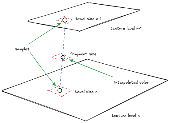
We then perform color sampling on these two texture maps, resulting in two colors. Finally, we interpolate or calculate a weighted average between these two colors. This calculation is based on how closely the fragment size matches the texels of the two selected textures.

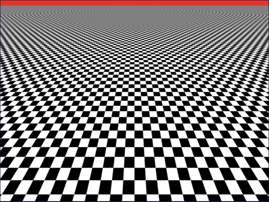
The result when mipmapping is applied is shown below. As we can observe, when the texture map is farther from our viewpoint, it gradually transitions to gray—a blend of black and white—rather than remaining strictly black or white. This gradual loss of detail aligns with our real-life visual experience when observing objects at a distance.

Improved Quality Due to Mipmapping

One extra step in implementing mipmapping with WebGPU is the need to manually create our mipmap using a shader. Users familiar with other graphics APIs like OpenGL may be accustomed to automatic mipmap generation for texture maps. However, in WebGPU, we must write code to accomplish this. Fortunately, the process is not overly complex. Let's examine the necessary code changes.

const textureDescriptor = {
    size: { width: imgBitmap.width, height: imgBitmap.height },
    format: 'rgba8unorm',
    mipLevelCount: Math.ceil(Math.log2(Math.max(imgBitmap.width, imgBitmap.height))),
    usage: GPUTextureUsage.TEXTURE_BINDING | GPUTextureUsage.COPY_DST | GPUTextureUsage.RENDER_ATTACHMENT
};
const texture = device.createTexture(textureDescriptor);
device.queue.copyExternalImageToTexture({ source: imgBitmap }, { texture }, textureDescriptor.size);

Note that when creating the checkerboard texture map, we're not utilizing our helper function for image-to-texture map conversion. Instead, we're manually defining the mipmap level count.

l = \lceil \log_2 max(w,h) \rceil

We calculate the mipmap level count using the equation shown above. This approach allows us to halve the width and height at each level until we reach the size of a single pixel.

Importantly, the usage flags for the texture include not only TEXTURE_BINDING but also COPY_DST and RENDER_ATTACHMENT. This configuration is necessary because we'll be using the same texture map for both reading and writing, as well as a render target during the mipmap generation process.

Let's now examine the shader-side modifications. You'll notice that we're utilizing two distinct shaders this time. One shader is dedicated solely to generating the mipmap for our texture, while the second shader is used for the actual rendering. We'll first analyze the mipmap shader, then proceed to discuss the JavaScript changes necessary for mipmap generation.

var<private> pos : array<vec2<f32>, 4> = array<vec2<f32>, 4>(
    vec2<f32>(-1.0, 1.0), vec2<f32>(1.0, 1.0),
    vec2<f32>(-1.0, -1.0), vec2<f32>(1.0, -1.0));

  struct VertexOutput {
    @builtin(position) position : vec4<f32>,
    @location(0) texCoord : vec2<f32>,
  };

  @vertex
  fn vs_main(@builtin(vertex_index) vertexIndex : u32) -> VertexOutput {
    var output : VertexOutput;
    output.texCoord = pos[vertexIndex] * vec2<f32>(0.5, -0.5) + vec2<f32>(0.5);
    output.position = vec4<f32>(pos[vertexIndex], 0.0, 1.0);
    return output;
  }

  @group(0) @binding(0) var imgSampler : sampler;
  @group(0) @binding(1) var img : texture_2d<f32>;

  @fragment
  fn fs_main(@location(0) texCoord : vec2<f32>) -> @location(0) vec4<f32> {
    return textureSample(img, imgSampler, texCoord);
  }

Following this, we'll explore how to sample the mipmap based on distance. The mipmap shader is relatively straightforward. We're employing the same technique we've encountered previously, where we define vertex data as an array rather than passing it from external sources.

It's important to note that any data defined outside a function scope must have a specified storage location. In this case, the position buffer is stored in private storage.

In the vertex shader, we derive the texture coordinates and positions based on the vertex index. Our goal is to generate a rectangle that covers the entire canvas or screen, effectively rendering the complete image across this area.

The fragment shader is straightforward, simply sampling the texture map based on the provided texture coordinates. In the JavaScript code, to create the mipmap, we first need to define a mipmap pipeline.

The process is relatively simple, but the key lies in the implementation. We begin by creating a texture map from the checkerboard image. Then, we use the same checkerboard texture map but target a different level as our render target. We render the texture map as a screen-aligned rectangle on the specified level, effectively shrinking the texture map. This process is repeated until all texture map levels are populated.

To use the texture as a render target, we need to create a view from the texture map. Unlike previous instances where we created views without parameters, here we provide two additional parameters:

let srcView = texture.createView({
    baseMipLevel: 0,
    mipLevelCount: 1
});
const sampler = device.createSampler({ minFilter: 'linear' });

// Loop through each mip level and renders the previous level's contents into it.
const commandEncoder = device.createCommandEncoder({});

for (let i = 1; i < textureDescriptor.mipLevelCount; ++i) {
    const dstView = texture.createView({
        baseMipLevel: i,  // Make sure we're getting the right mip level...
        mipLevelCount: 1, // And only selecting one mip level
    });

    const passEncoder = commandEncoder.beginRenderPass({
        colorAttachments: [{
            view: dstView, // Render pass uses the next mip level as it's render attachment.
            clearValue: { r: 0, g: 0, b: 0, a: 1 },
            loadOp: 'clear',
            storeOp: 'store'
        }],
    });

    // Need a separate bind group for each level to ensure
    // we're only sampling from the previous level.
    const bindGroup = device.createBindGroup({
        layout: uniformBindGroupLayout,
        entries: [{
            binding: 0,
            resource: sampler,
        }, {
            binding: 1,
            resource: srcView,
        }],
    });

    // Render
    passEncoder.setPipeline(mipmapPipeline);
    passEncoder.setBindGroup(0, bindGroup);
    passEncoder.draw(4);
    // what is a render pass;
    passEncoder.end();

    srcView = dstView;
}
device.queue.submit([commandEncoder.finish()]);

This process involves two texture views. If the source view points to level i of the texture, the target view will select level i+1, continuing until all levels are processed.

When creating a texture view, the baseMipLevel parameter specifies the render target level. Level 0 contains the original image, level 1 a shrunk version, and so on. The mipLevelCount is always set to 1, indicating that we process only one mipmap level at a time.

For the sampler, we use linear interpolation. This means that when shrinking the original image to generate our mipmap, we perform linear interpolation of the pixels. While this operation may slightly blur the image, a softer version of the texture map is actually desirable for objects viewed from a distance.

While this operation may slightly blur the image, a softer version of the texture map is actually beneficial for objects viewed from a distance.

We then create an encoder to generate the draw commands. The process involves drawing a series of rectangles, each corresponding to one level of the mipmap.

For each iteration, we progressively reduce the size of the target. We create a target that is one level above the source view of the texture map. This approach allows us to shrink the image incrementally. It's worth noting that there's no need to explicitly specify the width and height of each mipmap level - this is handled automatically, with both dimensions halving as the level increases.

We create our color attachment from the destination view and provide the source view for the binding group. The drawing process involves four indices. After each iteration, we reassign the destination view as the new source view, and the loop continues to generate the next mipmap level.

Once these commands are executed, the mipmap is fully generated and ready for use in normal rendering. The rendering process remains unchanged from our previous implementation. Importantly, the selection of appropriate mipmap levels and the interpolation between these levels are handled automatically by the graphics pipeline:

@group(0) @binding(2)
var t_diffuse: texture_2d<f32>;
@group(0) @binding(3)
var s_diffuse: sampler;

@fragment
fn fs_main(in: VertexOutput) -> @location(0) vec4<f32> {
    return textureSample(t_diffuse, s_diffuse, in.tex_coords) ;
}

However, there's an important caveat to consider: the textureSample function must meet the uniformity requirements (must be called within a uniform control flow). The concept of uniform control flow might be challenging to grasp at this point, and we'll explore it in more depth in later chapters. For now, we can simplify it as follows: a piece of code is in a uniform control flow if it will be executed regardless of the shader invocation. This means that no matter what shader inputs we provide, including uniforms and vertex attributes, that specific piece of code will always be executed.

Let's look at a counter-example that doesn't fulfill the uniformity requirement:

@group(0) @binding(2)
var t_diffuse: texture_2d<f32>;
@group(0) @binding(3)
var s_diffuse: sampler;

@fragment
fn fs_main(in: VertexOutput,  @builtin(front_facing) face: bool) -> @location(0) vec4<f32> {
    if (face) {
        return textureSample(t_diffuse, s_diffuse, in.tex_coords) ;
    } else {
        return vec4<f32>(0.0, 1.0, 0.0, 1.0); // Green for back-facing
    }
}

This code won't compile because it violates the uniformity requirement. The execution of textureSample depends on whether a fragment is front-facing or not, which means we can't guarantee its execution across all invocations.

If we want to return the texture map color only for front-facing fragments, the correct approach is to perform the texture sampling outside the conditional statement:

@group(0) @binding(2)
var t_diffuse: texture_2d<f32>;
@group(0) @binding(3)
var s_diffuse: sampler;

@fragment
fn fs_main(in: VertexOutput,  @builtin(front_facing) face: bool) -> @location(0) vec4<f32> {
    let c: vec4<f32> = textureSample(t_diffuse, s_diffuse, in.tex_coords);
    if (face) {
        return c;
    } else {
        return vec4<f32>(0.0, 1.0, 0.0, 1.0); // Green for back-facing
    }
}

While identifying uniformity issues by visual inspection of the code may seem challenging, fortunately, the WebGPU shader compiler is designed to report such problems. We'll dig deeper into the reasons behind these requirements in later chapters.

Mipmapping, while effective, has a limitation. In our previous example, we assumed that the sample rate for the texture should be uniform across both x and y directions. However, this isn't always the case. When viewing a texture at oblique angles, from the screen's perspective, the texture may be compressed along one direction more than another. In such situations, we need to apply different sample rates along different directions. This approach is known as anisotropic sampling, and it can significantly enhance rendering quality.

Implementing anisotropic sampling is relatively straightforward, though it does come with a trade-off in rendering speed. To enable it, we set maxAnisotropy > 1 when defining the sampler. This parameter represents the maximum ratio of anisotropy supported during filtering. To more clearly observe the effects of anisotropy, we can adjust the camera of the above example to a more oblique angle. Here's a comparison of the results before and after enabling anisotropic sampling:

The Sample Checker Board Rendered Without (Top) and With (Bottom) Anisotropic Sampling

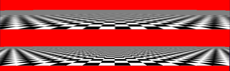
As you can see, anisotropic sampling provides a noticeable improvement in texture quality, especially at oblique angles. The top image shows the standard mipmapping result, while the bottom image demonstrates the enhanced detail and reduced distortion achieved through anisotropic sampling.

Implementing anisotropic sampling is left as an exercise for you to explore further.