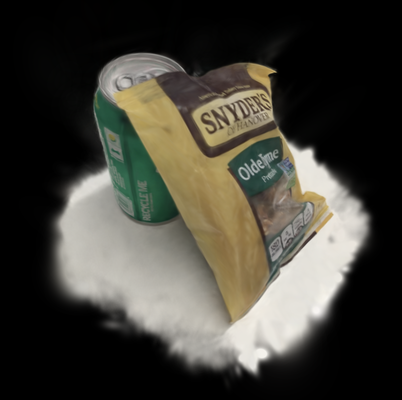
5.8 Gaussian Splatting

Gaussian Splatting has garnered significant attention since last year, particularly following this paper. This technique has piqued my interest due to its potential to become a standard approach for implementing 3D photography.

Traditional computer graphics predominantly represent 3D scenes using triangles, and GPU hardware is optimized for rendering large quantities of triangles efficiently. The quest for reconstructing a realistic 3D scene from a set of photos taken from different angles has been a vibrant research area. However, achieving photorealism remains a challenge. Triangles fall short when it comes to representing fuzzy, transparent, or non-distinctive objects like clouds or hair.

In recent years, there have been advancements in implicit 3D representations such as neural radiance fields. These methods can generate photorealistic results and handle non-distinctive objects well, albeit at the cost of intense computation and slow rendering speeds. Subsequently, researchers have been exploring new solutions that can bridge the gap between these approaches. Gaussian splatting emerges as a potential solution. However, this is a rapidly evolving field, with new methods coming out attempting to address some of the limitations of Gaussian splatting. Nevertheless, understanding Gaussian splatting deeply is worthwhile, as it may form the foundation for many future methods.

In this tutorial, we'll explore how to render Gaussian splats and make sense of its mathematics. Similar to other chapters, rather than focusing on mathematical rigor, I'd like to emphasize intuition, as I believe it is crucial for understanding complex concepts. For those interested in formal descriptions of the method, I'll recommend additional resources. I've also received invaluable assistance from the GaussianSplats3D reference implementation in Three.js. I highly recommend checking out this project.

Surface Splatting[SOURCE]

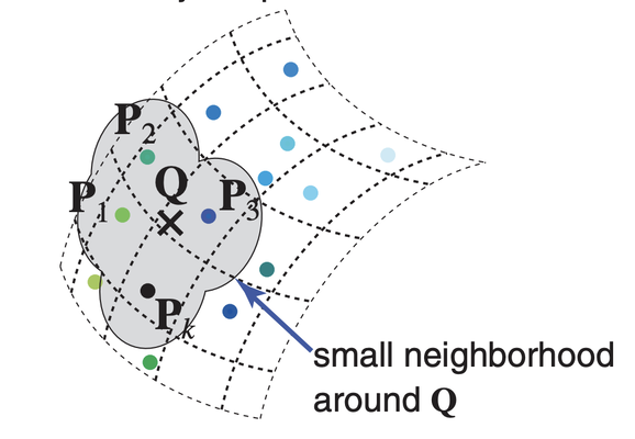
What is Gaussian Splatting? As previously mentioned, while triangles are the most commonly used graphics element, there has been a pursuit of using other primitives instead of triangles as the basis for rendering. Points, for example, have been another common choice. Points don't require explicit connectivity, making them handy when representing a 3D scene where connectivity is difficult to sort out, such as those captured using a 3D scanner or LiDAR. However, points don't have size. When viewed closely, points might not be dense enough to cover a surface. One idea for alleviating this problem is to render small disks, called surface splats, instead of points. Because a disk can have a size, tweaking their size can help cover the holes. The disks usually don't have a solid color but have a fading color on the edge defined by a Gaussian. This is useful to blend nearby disks to create a smooth transition.

Volume Rendered Fuzzy Object[SOURCE]

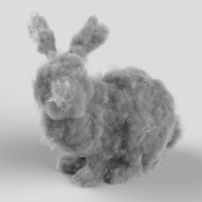
Another common choice is called volume rendering. A volume is a 3D grid of voxels, which can be viewed as 3D pixels that absorb light. We shoot out rays from the camera and test the intersection between the rays and the voxels, blending their color values along each ray. Voxel rendering excels in representing fuzzy surfaces, but the traditional way of storing a volume is very costly.

Gaussian splatting can be viewed as a hybrid of the two. Each rendering element is a 3D Gaussian function, or a blob. It has a position and a size, similar to a surface splat. But unlike a surface splat, a Gaussian splat also has a volume, not just in 2D. Moreover, a Gaussian splat has a shape. The basic shape is a sphere, but we can stretch and rotate it into an arbitrary ellipsoid. The color defined in a Gaussian splat fades too according to its defining Gaussian function, similar to a surface splat. Gaussian splatting combines the benefits of both aforementioned approaches. It doesn't require connectivity, it's sparse, and is capable of representing fuzzy surfaces.

Although Gaussian splatting gained popularity last year through this paper, the concept isn't new, as the rendering part was first mentioned in this paper. To summarize the process, given a scene with many Gaussian splats, we first perform a series of rotations and scalings on them, similar to what we do to vertices in the normal rendering process. Then, these splats are projected onto the screen as 2D Gaussians. Finally, they are sorted based on depth for applying front-to-back blending.

If you're finding it challenging to visualize this concept, I recommend watching the YouTube video linked above to gain a clearer understanding.

This chapter is by far the most complex. Therefore, we will take a step-by-step approach. Before diving into the rendering part, let's first cover some basics.

First, we'll discuss the data format for Gaussian splatting, as we will load data from these files for our demo. Second, we will render the loaded data as a point cloud. This will give us confidence that we have loaded the data correctly. Third, instead of rendering the full scene, we will render a single Gaussian splat. This is the most important part, as it will help us understand the underlying mathematics. Finally, we will combine everything we've learned, including the radix sorting algorithm from the previous chapter, to render a full scene.

This chapter focuses on the rendering of Gaussian splatting. However, I need to briefly cover how Gaussian splats are generated. Usually, a Gaussian splat scene is generated from photos taken from different angles. If you want to set it up and do it yourself, you can visit the official Gaussian splatting repository. Alternatively, you can use one of the online tools, such as Polycam, which generates the Gaussian splat scene for you after you upload your images.

There are two main data formats for Gaussian splats. One is the PLY file used for point clouds. The PLY file is very flexible, containing a human-readable header that describes the format of its content, followed by a binary section containing the actual data.

Another common format is the .splat file. This format is a simple binary of consecutive Gaussians. The format can be described as follows:

• XYZ - Position (Float32)

• XYZ - Scale (Float32)

• RGBA - colors (uint8)

• IJKL - quaternion/rot (uint8)

In this tutorial, we will use the PLY file generated by Polycam. Below is the header of our PLY file:

ply
format binary_little_endian 1.0
element vertex 81946
property float x
property float y
property float z
property float nx
property float ny
property float nz
property float f_dc_0
property float f_dc_1
property float f_dc_2
property float f_rest_0
...
property float f_rest_44
property float opacity
property float scale_0
property float scale_1
property float scale_2
property float rot_0
property float rot_1
property float rot_2
property float rot_3
end_header

The header is mostly understandable, but I want to explain some fields that are not so obvious. Here,f_{dc} represents the Gaussian's color, and rot is the rotation quaternion. Instead of parsing this file directly in JavaScript, we will preprocess the PLY file in C++ to generate an easy-to-load JSON file. We will use the happly project for this task, avoiding the need to write our own file parser.

happly::PLYData plyIn("../../../data/food.ply");
std::vector<float> opacity = plyIn.getElement("vertex").getProperty<float>("opacity");
std::vector<float> scale0 = plyIn.getElement("vertex").getProperty<float>("scale_0");
std::vector<float> scale1 = plyIn.getElement("vertex").getProperty<float>("scale_1");
std::vector<float> scale2 = plyIn.getElement("vertex").getProperty<float>("scale_2");
std::vector<float> rot0 = plyIn.getElement("vertex").getProperty<float>("rot_0");
std::vector<float> rot1 = plyIn.getElement("vertex").getProperty<float>("rot_1");
std::vector<float> rot2 = plyIn.getElement("vertex").getProperty<float>("rot_2");
std::vector<float> rot3 = plyIn.getElement("vertex").getProperty<float>("rot_3");
std::vector<float> x = plyIn.getElement("vertex").getProperty<float>("x");
std::vector<float> y = plyIn.getElement("vertex").getProperty<float>("y");
std::vector<float> z = plyIn.getElement("vertex").getProperty<float>("z");
std::vector<float> f_dc_0 = plyIn.getElement("vertex").getProperty<float>("f_dc_0");
std::vector<float> f_dc_1 = plyIn.getElement("vertex").getProperty<float>("f_dc_1");
std::vector<float> f_dc_2 = plyIn.getElement("vertex").getProperty<float>("f_dc_2");
std::ofstream outputFile;
outputFile.open("food.json");
outputFile << "[";
for (int i = 0; i < opacity.size(); ++i)
{

    const double SH_C0 = 0.28209479177387814;

    outputFile << "{\"p\":[" << x[i] << ", " << y[i] << ", " << z[i] << "]," << std::endl;
    outputFile << "\"r\":[" << rot0[i] << ", " << rot1[i] << ", " << rot2[i] << "," << rot3[i] << "]," << std::endl;
    outputFile << "\"c\":[" << (0.5 + SH_C0 * f_dc_0[i]) << ", " << (0.5 + SH_C0 * f_dc_1[i]) << ", " << (0.5 + SH_C0 * f_dc_2[i]) << "]," << std::endl;

    outputFile << "\"s\":[" << exp(scale0[i]) << ", " << exp(scale1[i]) << ", " << exp(scale2[i]) << "]," << std::endl;
    outputFile << "\"o\":" << (1.0 / (1.0 + exp(-opacity[i]))) << "}";

    if (i != opacity.size() - 1)
    {
        outputFile << "," << std::endl;
    }
}
outputFile << "]";

happly is a very easy-to-use library. All you need to do is supply a field name, and it will return a list of values for that field. Note that we need to perform some data conversions for scale and opacity. I couldn't find official documentation on these fields, so the formula comes from a reference source code.

However, I want to explain the conversion for colors. The equation might seem strange, especially the constant applied to each color channel. In many computer graphics problems, we need to model a complex function on a sphere. For example, for a 3D location in space, light can come from all directions with different intensities. We need to find a function that, given a 3D direction, returns a light intensity. This is a typical function defined on a sphere. Since the function can be complex, we probably won't find a simple form to represent it. One solution is to break it down into a summation of a series of simpler functions. This technique is called spherical harmonics. It is similar to the Fourier transform, but each component is a spherical function.

Spherical harmonics are important for Gaussian splatting to model highly reflective surfaces. For surfaces such as mirrors or chrome metal, their appearance can change based on the viewing angles.

A detailed explanation of spherical harmonics is beyond the scope of this book. The key takeaway is that the constant SH_{C0} is the first coefficient of the spherical harmonics formula. Despite deriving the color with spherical harmonics, we don't seem to relate the color to viewing directions, as the colors are also constant. This is correct; in our example, we assume a constant color for each Gaussian, meaning we can't model reflective surfaces well.

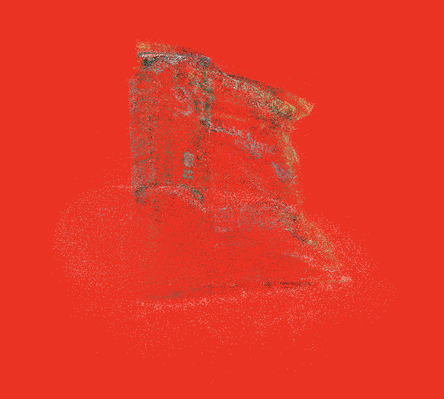
We want to be conservative and finish our rendering step by step. The first step is simply rendering the data as a point cloud. This should be straightforward for us now. Here is the shader code:

@group(0) @binding(0)
var<uniform> modelView: mat4x4<f32>;
@group(0) @binding(1)
var<uniform> projection: mat4x4<f32>;

struct VertexOutput {
    @builtin(position) clip_position: vec4<f32>,
    @location(0) color: vec4<f32>,
};

@vertex
fn vs_main(
    @location(0) inPos: vec3<f32>,
    @location(1) color: vec3<f32>,
    @location(2) opacity: f32
) -> VertexOutput {
    var out: VertexOutput;
    out.color = vec4<f32>(color, opacity);
    out.clip_position = projection * modelView * vec4<f32>(inPos, 1.0);
    return out;
}

@fragment
fn fs_main(in: VertexOutput) -> @location(0) vec4<f32> {
    return in.color;
}

And here is the rendering result:

Visualizing the Point Cloud

To understand how to render a Gaussian splat, we need to be familiar with the geometric interpretation of a 3D Gaussian function. For that, I recommend this document. I will skip the details and summarize what's useful for our implementation.

A 3D Gaussian is defined by two parameters: a centroid and a 3x3 covariance matrix. Intuitively, the centroid is the position of a Gaussian, and the covariance matrix defines the shape of the Gaussian (an ellipsoid).

\mathcal{N}(\mu, \sigma^2)

If we consider 1D Gaussians, they are defined by a mean \mu and a variance \sigma^2. In this context, the mean \mu dictates the center of the Gaussian on the x-axis, while \sigma^2 determines its spread or shape.

1D Gaussians of Different Means and Variances[SOURCE]

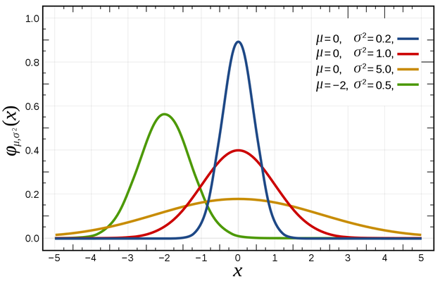
The same principle extends to 2D and 3D Gaussians, where they are defined by a mean \mu (or centroid) and a covariance matrix \Sigma. In 2D, the covariance \Sigma is a 2x2 matrix, and in 3D, it is a 3x3 matrix. The covariance matrix holds geometric significance, defining the ellipsoidal shape of the Gaussian.

\mathcal{N}(\mu, \Sigma)

Below is an illustration showing various 2D Gaussian shapes and their corresponding covariances.

2D Gaussian Shapes and Their Covariances[SOURCE]

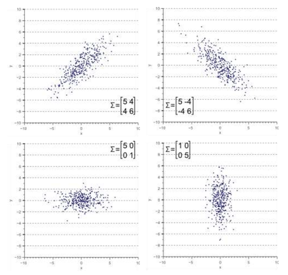
We can shift the centroid to adjust a Gaussian's position, and we can also rotate and scale the covariance matrix to modify its shape. This process is akin to applying a model-view matrix to vertices during rendering, although the mathematical operations involved are not identical.

The fundamental insight from the geometric interpretation outlined in the document is that the covariance matrix \Sigma specifies a rotation and scaling transformation that morphs a standard Gaussian with the identity matrix \mathbf I as its covariance into an ellipsoidal shape. Let this transformation be represented by a 3x3 matrix \textit{T}; it can be factored into a product of a 3x3 rotation matrix \textit{R} and a scaling matrix \textit{S}. Thus:

\begin{aligned} \Sigma &= \textit{T} \textit{I} \textit{T}^\top \\ \Sigma &= \textit{R} \textit{S} (\textit{R} \textit{S})^\top \\ \Sigma &= \textit{R} \textit{S} \textit{S}^\top \textit{R}^\top \\ \end{aligned}

Additionally, if we wish to apply an additional transformation \textit{V} to the covariance matrix, we can do so using the formula \Sigma^\prime = \textit{V} \Sigma \textit{V}^\top. This is crucial for tasks such as implementing projection of the 3D covariance into 2D space.

Before delving into rendering Gaussian splats, it's crucial to establish a ground truth. Debugging graphics programs can be challenging, so visualizing the rendering result against this ground truth is essential to ensure the implementation's correctness. There are two primary methods to create the ground truth:

1. Generate a point cloud from a Gaussian distribution, where the Gaussian value serves as the sample density.

2. Deform a sphere into an ellipsoid based on the same transformation defined by the Gaussian's covariance matrix.

Once the Gaussian splat has been rendered, we anticipate seeing it overlap with the ground truth, providing a visual confirmation of the accuracy of the implementation.

In this post, I'll use the first method. Python offers excellent support for point sampling, so I'll begin by implementing a helper program in Python to sample points from a Gaussian distribution and save the result to a file. Then, I'll render these points using WebGPU.

import numpy as np
import matplotlib.pyplot as plt
from mpl_toolkits.mplot3d import Axes3D
import codecs, json 

# Define the parameters of the Gaussian function
mu = [10, 10, 10]
sigma = [[2, 2, 0], [0, 1, 0], [2, 0, 1]]

cov = [[0.46426650881767273, -0.6950497627258301, -0.7515625953674316],
       [ -0.6950497627258301, 2.0874688625335693, 1.7611732482910156],
       [ -0.7515625953674316, 1.7611732482910156, 1.7881864309310913]]



# Generate the data
X = np.random.multivariate_normal(mu, cov, 10000)

json.dump(X.tolist(), codecs.open('points.json', 'w', encoding='utf-8'), 
          separators=(',', ':'), 
          sort_keys=True, 
          indent=4)

The code is straightforward. The key line is np.random.multivariate_normal(mu, cov, 10000), which samples 10,000 points from a multivariate normal distribution (the Gaussian). Then, we save their positions in a JSON file.

Point Samples Visualized as a Point Cloud

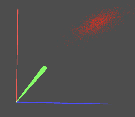
The covariance matrix used in the program above may appear arbitrary. I will provide an explanation of how these values were determined later in this post.

Now, let's define the single Gaussian splat we intend to render. Since the specific Gaussian splat doesn't matter for our purposes, we will simply select one at random. In this example, I've chosen a rotation represented by a quaternion of (0.601, 0.576, 0.554, 0.01) and a scaling vector of (2.0, 0.3, 0.5). Quaternions and scaling vectors are used because they are the information typically stored in a Gaussian splat file.

The first step involves deriving the rotation matrix and the scaling matrix to reconstruct the covariance matrix. For this task, we will utilize the glMatrix library.

const rot = glMatrix.quat.fromValues(0.601, 0.576, 0.554, 0.01);
let scale = glMatrix.mat4.fromScaling(glMatrix.mat4.create(), glMatrix.vec4.fromValues(2.0, 0.3, 0.5));
scale = glMatrix.mat3.fromMat4(glMatrix.mat3.create(), scale);
const rotation = glMatrix.mat3.fromQuat(glMatrix.mat3.create(), rot);

Then, according to equation 3, the covariance matrix can be derived as follows:

const T = glMatrix.mat3.multiply(glMatrix.mat3.create(), rotation, scale);

const T_transpose = glMatrix.mat3.transpose(glMatrix.mat3.create(), T);

this.covariance = glMatrix.mat3.multiply(glMatrix.mat3.create(), T, T_transpose);

The covariance matrix hardcoded in the Python sampling function is identical to the one calculated here.

During rendering, we update the model-view matrix based on the camera. Using this model-view matrix and the projection matrix, our goal is to accurately project the covariance matrix onto the screen plane, converting the 3D Gaussian into a 2D Gaussian.

The first step is to obtain the model-view matrix from the camera and convert it into a 3x3 matrix (the upper-left 3x3 corner). In vertex transformation with homogeneous coordinates, a 4x4 matrix is constructed for translation, with the offset values assigned to the last column of the matrix. However, when dealing with the 3x3 covariance matrix, we cannot perform translation, only rotation and scaling. Therefore, to obtain a 3x3 model-view matrix, we simply use the upper-left 3x3 corner. This is in contrast to billboarding, where the 3x3 upper-left corner is assigned the 3x3 identity matrix to remove rotation and scaling.

const W = glMatrix.mat3.transpose(glMatrix.mat3.create(), glMatrix.mat3.fromMat4(glMatrix.mat3.create(), arcballModelViewMatrix));

The second step involves performing perspective projection, which is akin to applying the projection matrix. In computer graphics, applying perspective projection transforms coordinates from either camera space or eye space into clip space. Prior to this transformation, the visible space is enclosed within a view frustum, which is a 3D trapezoidal volume. After the transformation, the visible space is represented as a cubic volume.

Projection Turns the View Frustum Into a Cubical Space[SOURCE]

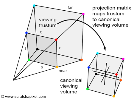
However, it's important to note that perspective transformation is not affine, which means that the original ellipsoidal shape will be warped once projected.

Warping Caused by Perspective Projection[SOURCE]

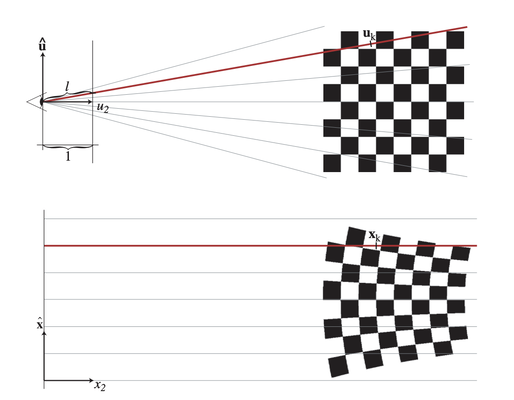
Since non-affine transformations cannot be represented as a 3x3 matrix and applied directly to the covariance matrix, our objective is to find an approximation that can transform the Gaussian in a manner that simulates the projection.

Illustration of Approximated Projection. Lower Left: Approximated Projection Doesn't Warp the Shape. Lower Right: Original Projection Would Warp the Shape.[SOURCE]

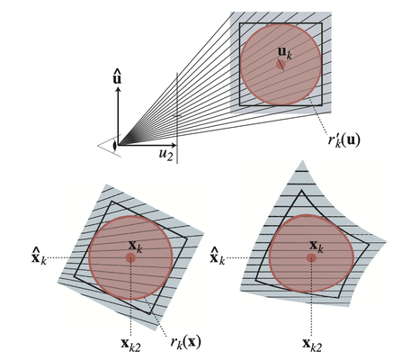
To approximate this transformation, we first consider how a point is projected onto the screen.

Perspective Projection of One Point to the Screen Plan[SOURCE]

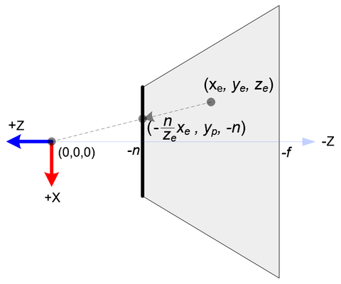
Given a point (x_e, y_e, z_e) in camera space to be projected onto the near plane at z=n, the projection can be calculated as follows:

\begin{aligned} x_p &= \frac{-n x_e}{z_e}\\ y_p &= \frac{-n y_e}{z_e}\\ z_p &= - || (x_e, y_e, z_e)^\top ||\\ \end{aligned}

This mapping from (x_e, y_e, z_e) to (x_p, y_p, z_p) is not affine and cannot be represented by a 3x3 matrix. According to the paper referenced here, we can approximate this transformation using the first two terms of the Taylor expansion of the mapping function: v_p + J(v-v_c), where v_p is the projected centroid of the Gaussian, and J is the Jacobian or the first-order derivative.

The concept of Taylor expansion, while its name might seem daunting, is actually quite straightforward. Let's illustrate it using a 1D unknown function y = f(x). Our aim is to estimate the function near a specific input point x_0. When we focus on a very small window around x_0, the function can be approximated by a straight line. This line can be obtained by calculating the derivative of the function f. Therefore, the value of f(x) where x is close to x_0 can be approximated by \bar{y} = f(x_0) + f^\prime(x_0)(x - x_0).

In our projection scenario, f(x_0) represents the projected position of the Gaussian's centroid, which we can easily calculate using the model-view matrix and the centroid position. f^\prime(x_0) corresponds to the Jacobian matrix, which we will use to transform the covariance matrix.

The Jacobian matrix (transposed) can be calculated as follows:

\begin{pmatrix} \frac{d x_p}{d x_e} & \frac{d y_p}{d x_e} & \frac{d z_p}{d x_e}\\ \frac{d x_p}{d y_e} & \frac{d y_p}{d y_e} & \frac{d z_p}{d y_e}\\ \frac{d x_p}{d z_e} & \frac{d y_p}{d z_e} & \frac{d z_p}{d z_e}\\ \end{pmatrix}

Based on equation 4, we can calculate the Jacobian matrix as follows:

\begin{pmatrix} -\frac{n}{z_e} & 0 & 0\\ 0 & -\frac{n}{z_e} & 0\\ \frac{x_e}{z_e^2} & \frac{y_e}{z_e^2} & 0\\ \end{pmatrix}

The last column should not be all zeros, but in our reference code, the last column is indeed set to zeros. I believe the reason for this is that for the projection of Gaussians, we can effectively remove the depth information by assuming z_p is a constant. This is because we do not need depth testing for Gaussians; instead, we will sort them from front to back and render them in that order.

Here is how the Jacobian matrix (in column-major order) is calculated in the code, based on the perspective projection matrix:

const focal = {
    x: projectionMatrix[0] * devicePixelRatio * renderDimension.x * 0.5,
    y: projectionMatrix[5] * devicePixelRatio * renderDimension.y * 0.5
}

const viewCenter = glMatrix.vec4.transformMat4(glMatrix.vec4.create(), glMatrix.vec4.fromValues(10, 10, 10, 1.0), arcballModelViewMatrix);

const s = 1.0 / (viewCenter[2] * viewCenter[2]);

const J = glMatrix.mat3.fromValues(
    -focal.x / viewCenter[2], 0., (focal.x * viewCenter[0]) * s,
    0., -focal.y / viewCenter[2], (focal.y * viewCenter[1]) * s,
    0., 0., 0.
);

The focal vector can be calculated by extracting the first and sixth elements from the projection matrix. These elements represent the horizontal and vertical arctangents of the half field of view. By multiplying them with the half width and half height of the canvas, respectively, we obtain the distance from the camera to the near plane. In theory, both focal.x and focal.y should be equal.

With both the 3x3 model-view matrix W and the Jacobian matrix J, we can now update our covariance as follows:

const W = glMatrix.mat3.transpose(glMatrix.mat3.create(), glMatrix.mat3.fromMat4(glMatrix.mat3.create(), arcballModelViewMatrix));
const T = glMatrix.mat3.multiply(glMatrix.mat3.create(), W, J);

let new_c = glMatrix.mat3.multiply(glMatrix.mat3.create(), glMatrix.mat3.transpose(glMatrix.mat3.create(), T), glMatrix.mat3.multiply(glMatrix.mat3.create(), this.covariance, T));

With the updated covariance, we extract its 2x2 upper left corner, which represents the covariance for the projected 2D Gaussian. Next, we need to recover two basis vectors from the 2D Gaussian, which correspond to the eigenvectors of the top two eigenvalues.

This is calculated using the following formula:

const cov2Dv = glMatrix.vec3.fromValues(new_c[0], new_c[1], new_c[4]);

let a = cov2Dv[0];
let b = cov2Dv[1];
let d = cov2Dv[2];

let D = a * d - b * b;
let trace = a + d;
let traceOver2 = 0.5 * trace;
let term2 = Math.sqrt(trace * trace / 4.0 - D);
let eigenValue1 = traceOver2 + term2;
let eigenValue2 = Math.max(traceOver2 - term2, 0.00); // prevent negative eigen value

const maxSplatSize = 1024.0;
let eigenVector1 = glMatrix.vec2.normalize(glMatrix.vec2.create(), glMatrix.vec2.fromValues(b, eigenValue1 - a));
// since the eigen vectors are orthogonal, we derive the second one from the first
let eigenVector2 = glMatrix.vec2.fromValues(eigenVector1[1], -eigenVector1[0]);

let basisVector1 = glMatrix.vec2.scale(glMatrix.vec2.create(), eigenVector1, Math.min(Math.sqrt(eigenValue1) * 4, maxSplatSize));
let basisVector2 = glMatrix.vec2.scale(glMatrix.vec2.create(), eigenVector2, Math.min(Math.sqrt(eigenValue2) * 4, maxSplatSize));

In the vertex shader code, we utilize the basis vectors to construct a screen-aligned quad. The long edge of the quad should be parallel to the first basis vector, while the short edge should be parallel to the second eigenvector.

var clipCenter:vec4<f32> = projection * modelView * pos;

var ndcCenter:vec3<f32> = clipCenter.xyz / clipCenter.w;

var ndcOffset:vec2<f32> = vec2(inPos.x * basisVector1 + inPos.y * basisVector2) * basisViewport;

out.clip_position = vec4<f32>(ndcCenter.xy + ndcOffset, ndcCenter.z, 1.0);

In the shader code, we manually calculate the position of the centroid in Normalized Device Coordinates (NDC). Since NDC has a range of [-1, 1] for both the x and y axes, we need to scale the ndcOffset. Because the Jacobian is calculated using pixels as the unit length, we need to scale it down by (\frac{w}{2},\frac{h}{2}), where w and h are the width and height of the canvas, respectively.

Gaussian Rendering Result Overlapping the Ground Truth Point Cloud

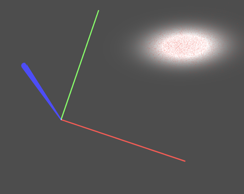
The rendering result is shown above. As we can see, the Gaussian is correctly rendered, overlapping perfectly with the ground truth point cloud.

Now that we have rendered a single Gaussian splat, we need to extend our program to render the entire point cloud. Because our Gaussian splats are semi-transparent, we need to enable blending and render them in front-to-back order.

This is where our previous radix sort algorithm comes into play. The process is as follows: first, we calculate the projected basis and the distance to the camera for each splat. This process is identical to what we explained earlier, but we will implement it in a compute shader and apply it to all splats at once. Then, we use GPU radix sorting to reorder the splats from front to back. Finally, we iterate through the ordered Gaussian splats and render them in sequence.

Now let's look at how to efficiently calculate the distances from the camera to the splats:

// given centroids, covariance, modelView, projection;
// compute 2d basis, distance
@binding(0) @group(0) var<storage, read> centroid :array<vec3<f32>>;
@binding(1) @group(0) var<storage, read> covariance: array<vec3<f32>>;
@binding(2) @group(0) var<storage, read_write> basis: array<vec4<f32>>;
@binding(3) @group(0) var<storage, read_write> distance: array<u32>;
@binding(4) @group(0) var<storage, read_write> id: array<u32>;
@binding(5) @group(0) var<uniform> splatCount: u32;
@binding(6) @group(0) var<storage, read_write> readback: array<vec4<f32>>;

@binding(0) @group(1) var<uniform> modelView: mat4x4<f32>;
@binding(1) @group(1) var<uniform> projection: mat4x4<f32>;
@binding(2) @group(1) var<uniform> screen: vec2<f32>;

@compute @workgroup_size(256)
fn main(@builtin(global_invocation_id) GlobalInvocationID : vec3<u32>,
  @builtin(local_invocation_id) LocalInvocationID: vec3<u32>,
  @builtin(workgroup_id) WorkgroupID: vec3<u32>) {
    var gid = GlobalInvocationID.x;

    if (gid < splatCount) {
        var covarianceFirst = covariance[gid*2];
        var covarianceSecond = covariance[gid*2+1];

        var covarianceMatrix: mat3x3<f32> = mat3x3(
            covarianceFirst.x,
            covarianceFirst.y,
            covarianceFirst.z,
            covarianceFirst.y,
            covarianceSecond.x,
            covarianceSecond.y,
            covarianceFirst.z,
            covarianceSecond.y,
            covarianceSecond.z);

        var modelView3x3:mat3x3<f32> = transpose( mat3x3<f32>(modelView[0].xyz, modelView[1].xyz, modelView[2].xyz));

        var cameraFocalLengthX:f32 = projection[0][0] *
        screen.x * 0.5;
        var cameraFocalLengthY:f32 = projection[1][1] *
        screen.y * 0.5;

        var center:vec4<f32> = vec4(centroid[gid], 1.0);

        var viewCenter:vec4<f32> =   modelView * center;
        var s:f32 = 1.0 / (viewCenter.z * viewCenter.z);

        var J = mat3x3<f32>(
            cameraFocalLengthX / viewCenter.z, 0.0, -(cameraFocalLengthX * viewCenter.x) * s,
            0.0, cameraFocalLengthY / viewCenter.z, -(cameraFocalLengthY * viewCenter.y) * s,
            0.0, 0.0, 0.0
        );

        var T:mat3x3<f32> =  modelView3x3 * J ;

        var T_t:mat3x3<f32> = transpose(T);
    
        var new_c:mat3x3<f32> =  T_t * covarianceMatrix * T;
        
        var cov2Dv:vec3<f32> = vec3<f32>(new_c[0][0] , new_c[0][1], new_c[1][1]);
          
        var a:f32 = cov2Dv.x;
        var b:f32 = cov2Dv.y;
        var d:f32 = cov2Dv.z;

        var D:f32 = a * d - b * b;
        var trace:f32 = a + d;
        var traceOver2:f32 = 0.5 * trace;
        var term2:f32 = sqrt(trace * trace / 4.0 - D);
            
        var eigenValue1:f32 = traceOver2 + term2;
        var eigenValue2:f32 = max(traceOver2 - term2, 0.0);

        const maxSplatSize:f32 = 1024.0;
        var eigenVector1:vec2<f32> = normalize(vec2<f32>(b, eigenValue1 - a));
        var eigenVector2:vec2<f32> = vec2<f32>(eigenVector1.y, -eigenVector1.x);
  
        var basisVector1:vec2<f32> = eigenVector1 * min(sqrt(eigenValue1)*4, maxSplatSize);
        var basisVector2:vec2<f32> = eigenVector2 * min(sqrt(eigenValue2)*4, maxSplatSize);
        readback[gid] = vec4<f32>(basisVector1,basisVector2);
        var dis:vec4<f32> = projection * modelView * center;
        distance[gid] = u32(((dis.z / dis.w+1.0)*0.5) * f32(0xFFFFFFFF >> 8));     
        basis[gid] = vec4<f32>(basisVector1, basisVector2);
    } else {
        distance[gid] = 0xFFFFFFFF;
    }
    id[gid] = gid;
}

Most of the code has been explained before. The difference here is that we also incorporate the calculation of the distances from the camera to the splats. The calculation itself is the same as applying a projection matrix.

Here are some important details to pay attention to. First, we scale and convert the distance value to an integer: distance[gid] = u32(dis.z / dis.w * f32(0xFFFFFFFF >> 8));. The reason for this is that our radix sorting can only process integers. Second, for padding splats, we set their distance to the maximum possible value: distance[gid] = 0xFFFFFFFF;. We can't guarantee that the number of splats is always a multiple of 512. Hence, we usually need to pad the input array at the end. For these padded dummy splats, we simply give them the maximum possible distance so that after sorting, they will be located at the end of the array, allowing us to easily truncate them.

Next comes the sorting part. It is almost the same as what we have seen before. The difference lies in the shuffling part; because our array is more complex, we have to shift more data than a single integer. However, the principle remains the same.

Finally, with the splats sorted, we apply front-to-back rendering:

encode(encoder) {
    encoder.setPipeline(this.splatPipeline);
    encoder.setBindGroup(0, this.splatUniformBindGroup0);
    encoder.setBindGroup(1, this.splatUniformBindGroup1)
    encoder.setVertexBuffer(0, this.splatPositionBuffer);
    encoder.setVertexBuffer(1, this.idBuffer);
    for (let i = this.actualSplatSize - 1; i >= 0; --i) {
        encoder.draw(4, 1, 0, i);
    }
}

You may ask why we can't use the instanced rendering technique here instead of a for loop. The reason is that we have to maintain the rendering order to ensure correct blending. With instanced rendering, there is no guarantee of the rendering order since the splats will be drawn in parallel.

Rendered Gaussian Splatting Scene