1.9 Implementing Cameras

In our exploration of computer graphics, we've primarily focused on rendering 2D objects until now. It's time to venture into the realm of 3D rendering and introduce the concept of a camera into our code. You might be surprised to learn that the camera isn't a built-in feature defined within the GPU pipeline or the WebGPU API standard. Instead, we'll craft our own camera by simulating a pinhole camera using model-view transformations and projection onto our vertices, achieved through matrix multiplications.

Before diving into the camera implementation, let's first examine the coordinate systems used by the graphics pipeline and the methods for converting between them. While not every coordinate system is part of the WebGPU specification, these represent the most common approaches to handling coordinate conversion.

Handedness

To understand any coordinate system, we must first grasp the concept of handedness. A 3D coordinate system can be either left-handed or right-handed. Imagine facing the xy plane with the x-axis pointing to the right and the y-axis pointing up. The choice of handedness determines the direction of the z-axis.

The Left-Handed Coordinates vs. The Right-Handed Coordinates

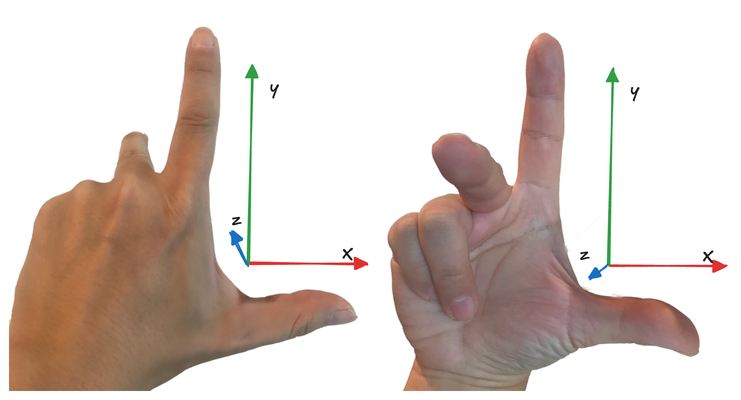
In a right-handed system, if you align your right hand's thumb with the positive x direction and your index finger with the positive y direction, your middle finger will point in the positive z direction. Conversely, in a left-handed system, using your left hand in the same manner will indicate the positive z direction.

To visualize this, picture your computer screen as the xy coordinate plane. In a right-handed system, the z-axis points towards you, while in a left-handed system, it points into the screen.

The choice of handedness is a convention you establish for your program. While the specific system doesn't matter, understanding the concept is crucial for making sense of the mathematics in your application. The handedness of certain coordinates is determined by the WebGPU specification, while for others, it depends on your chosen math library. In our case, we're using the glMatrix library, which adopts a right-handed system to align with OpenGL conventions.

Local coordinates

Most 3D models are created in their own coordinate system, known as local coordinates. For instance, in video game development, a 3D character is typically modeled in a 3D application using its own coordinate system. For convenience, the character might be positioned at the origin in this local space.

World coordinates

A single model doesn't create an entire game world. Often, we need to load numerous 3D models and construct a 3D scene from them. In most 3D applications, models are dynamic—you can move, rotate, and scale them within the 3D scene. Consequently, we can't rely solely on each model's local coordinates. We need to transform their coordinate systems into a unified one.

At this stage, our primary concern is the translation, rotation, and scaling of the models and their relative positions. We can choose any point in 3D space as the world's origin and offset all models accordingly. Regardless of which coordinate system you designate as the world coordinate system, the conversion from a model's local coordinates to world coordinates should be accomplished through a single matrix multiplication. This matrix is called the model matrix. After this conversion, all models in the scene should use the same coordinate system.

View coordinates

Our ultimate goal is to project the 3D scene onto a 2D view plane. This projection is calculated relative to the viewpoint, which is the location of the camera. To simplify this process, we convert the coordinate system once more, creating what's known as the view coordinate system.

In this new system, the camera's position becomes the origin. The y-axis points upward, the x-axis points to the right, and in our right-handed coordinate system, the z-axis points towards the camera. Consequently, the negative z-axis extends into the scene. This transformation allows us to calculate the projection from the camera's perspective more easily.

Projection

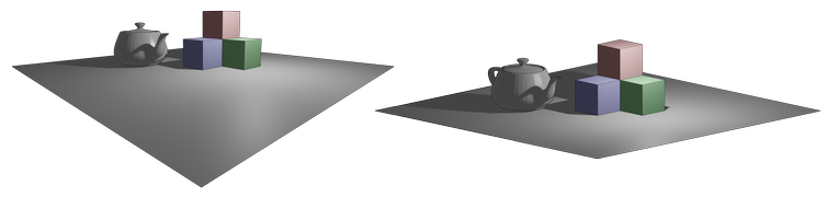
Projection is the process of transforming our 3D scene onto a 2D plane, and there are two primary types: perspective and orthogonal.

Perspective projection mimics how we perceive depth in the real world, where objects farther from the viewer appear smaller. This creates a sense of depth and realism in rendered scenes. Orthogonal projection, on the other hand, maintains object size regardless of distance. While less common in realistic rendering, orthogonal projection has valuable applications in technical drawings and certain types of games.

In this discussion, we'll focus on perspective projection, reserving orthogonal projection for a future exploration. The following image illustrates the key difference between these two projection types:

Perspective Projection (Left) vs. Orthogonal Projection (Right)

To model our camera, we use a simple pinhole model. In this model, the visible volume forms a shape called a frustum - essentially a truncated pyramid. The front face of this frustum can be thought of as our screen or view plane.

With a Pin-Hole Camera Model, the Visible Volume Is a Trapezoidal Prism, Called the View Frustum

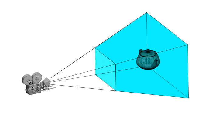
The primary objective of perspective projection is to transform this trapezoidal frustum into a cuboid. In this transformation, both the front and back faces of the frustum are adjusted to the same size. Specifically, after projection, both the front and back planes, as well as the z-range, must fall within the range of [-1, 1]. In other words, our projection deforms the original visible volume into a cube with a side length of 2.

This resulting cuboid exists in what we call Normalized Device Coordinates (NDC). The NDC system is a standardized 3D space that simplifies the final stages of rendering, regardless of the original scene's scale or the specific projection used.

Projection Converts the View Frustum in the View Coordinates Into Normalized Device Coordinates

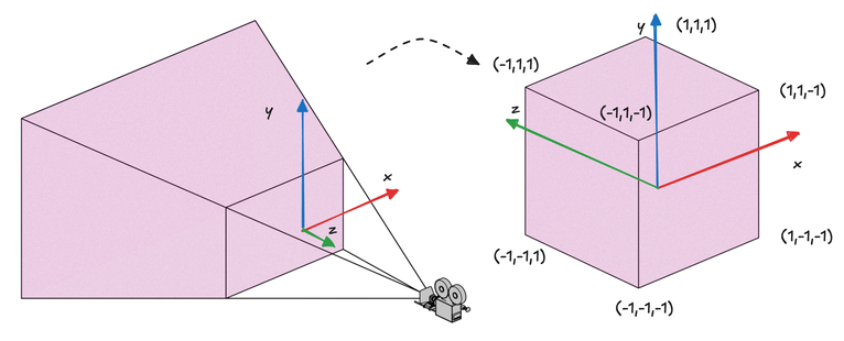
Normalized Device Coordinates (NDC) represent a standardized 3D space enclosed by the points (-1,-1,-1) and (1,1,1). The transformation from view coordinates to NDC, accomplished through the projection process, is illustrated in the image above. It's crucial to note a significant change that occurs during this transformation: while the view coordinates are right-handed, the resulting NDC system becomes left-handed, with the positive z-axis now pointing away from the camera.

This shift in handedness is a critical point of distinction. Prior to NDC, all the coordinate systems we've discussed are not strictly defined by the WebGPU specification, allowing developers the flexibility to choose their preferred handedness. However, the NDC system is explicitly defined in the WebGPU spec, requiring strict adherence. The projection process facilitates this transition from a right-handed to a left-handed system by essentially flipping the z-axis, an operation conceptually similar to mirroring.

Like other transformations we've encountered, projection can be achieved through a single matrix multiplication. However, deriving this projection matrix is not as straightforward as it might seem at first glance. To understand its construction, let's approach it step by step.

Project of a Point E in the View Coordinates to the Near Plane

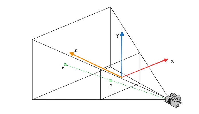
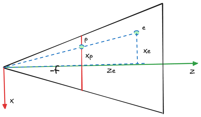
Let's begin by focusing on the x-axis. We'll project point e onto the near plane, resulting in point p. The x and y coordinates of p must then be mapped to the range [-1, 1] for use in NDC.

Top View of the View Coordinates

We can establish the following relationship:

\begin{aligned} \frac{x_p}{x_e} &= \frac{-n}{z_e} \\ x_p &= \frac{-n*x_e}{z_e} \end{aligned}

Here, n represents the focal length (or the near plane distance) of our pinhole camera model. The y-coordinate follows an identical relationship:

\begin{aligned} \frac{y_p}{y_e} &= \frac{-n}{z_e} \\ y_p &= \frac{-n*y_e}{z_e} \end{aligned}

While (x_p, y_p) gives us the coordinates of the projected point p on the near plane, these are not yet the NDC coordinates. To comply with NDC requirements, we need to map these coordinates to the range [-1, 1]. This mapping is a linear transformation:

Linear Relationship Between the Coordinates of P to Its NDC

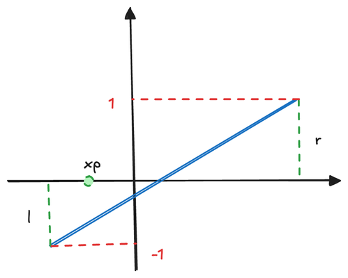
\begin{aligned} x_{ndc} &= \frac{1--1}{r-l}*x_p + \beta_{1} \\ y_{ndc} &= \frac{1--1}{t-b}*y_p + \beta_{2} \end{aligned}

Here, r and l represent the right and left boundaries of the near plane, while t and b denote the top and bottom boundaries. When p is at the center of the near plane (i.e., at (\frac{r+l}{2},\frac{t+b}{2})), (x_{ndc}, y_{ndc}) should also be at the center (0, 0). Using this relationship, we can determine \beta_{1} and \beta_{2}:

\begin{aligned} \beta_{1} &= - \frac{1--1}{r-l}*\frac{r+l}{2} = - \frac{r+l}{r-l} \\ \beta_{2} &= - \frac{1--1}{t-b}*\frac{t+b}{2} = - \frac{t+b}{t-b} \end{aligned}

Thus, our equations become:

\begin{aligned} x_{ndc} &= \frac{1--1}{r-l}*x_p - \frac{r+l}{r-l} \\ &= \frac{1--1}{r-l}* \frac{-n*x_e}{z_e} - \frac{r+l}{r-l} \\ &= \frac{-2n*x_e}{z_e*(r-l)} - \frac{r+l}{r-l} \\ &= - \frac{\frac{2n*x_e}{r-l} + \frac{r+l}{r-l}}{z_e} \\ y_{ndc} &= \frac{1--1}{t-b}*y_p - \frac{t+b}{t-b} \\ &= \frac{1--1}{t-b}* \frac{-n*y_e}{z_e} - \frac{t+b}{t-b} \\ &= \frac{-2n*y_e}{z_e*(t-b)} - \frac{t+b}{t-b} \\ &= - \frac{\frac{2n*y_e}{t-b} + \frac{t+b}{t-b}}{z_e} \end{aligned}

Now, let's express this transformation in matrix form:

\begin{pmatrix} \frac{2n}{r-l} & 0 & \frac{r+l}{r-l} & 0 \\ 0 & \frac{2n}{t-b} & \frac{t+b}{t-b} & 0 \\ 0 & 0 & A & B \\ 0 & 0 & -1 & 0 \end{pmatrix} \times \begin{pmatrix} x_e \\ y_e \\ z_e \\ 1 \end{pmatrix}

Note that to calculate x_{ndc} and y_{ndc}, we need to divide by -z_e as the final step. We achieve this by utilizing the homogeneous coordinates' scaling factor w_{ndc} = -z_e. This approach allows us to incorporate the division into our matrix multiplication, which is crucial since direct element-wise division isn't possible in matrix multiplication.

The final piece of our projection puzzle is mapping z_e to z_{ndc}. Unlike the linear mapping from x_e to x_p, the relationship between z_e and z_p is non-linear. Although we could find a linear mapping between them, we opt for a different approach to accommodate our matrix multiplication format. Let's derive the values for A and B in our projection matrix:

\begin{aligned} z_{ndc} &= \frac{A*z_e + B}{-z_e} \\ \frac{-An+B}{n} &= -1 \\ \frac{-Af+B}{f} &= 1 \end{aligned}

Here, -n and -f represent the near and far plane distances, respectively. Solving for A and B:

\begin{aligned} A &= - \frac{f+n}{f-n}\\ B &= - \frac{2fn}{f-n} \\ z_{ndc} &= \frac{- \frac{f+n}{f-n}*z_e - \frac{2fn}{f-n}}{-z_e} \end{aligned}

Now we can express the complete projection calculation as a single matrix multiplication:

\begin{pmatrix} \frac{2n}{r-l} & 0 & \frac{r+l}{r-l} & 0 \\ 0 & \frac{2n}{t-b} & \frac{t+b}{t-b} & 0 \\ 0 & 0 & - \frac{f+n}{f-n} & - \frac{2fn}{f-n} \\ 0 & 0 & -1 & 0 \end{pmatrix} \times \begin{pmatrix} x_e \\ y_e \\ z_e \\ 1 \end{pmatrix}

It's important to note that the mapping between z_e and z_{ndc} is non-linear. To better understand this relationship, let's visualize it with a plot, assuming f = 50 and n = 10:

Plot the Mapping From Ze to Zndc

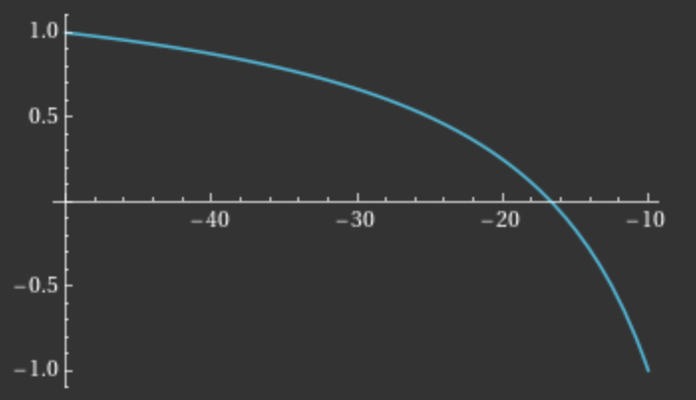
This graph reveals an interesting property: as we move from the far plane to the near plane, the rate of change in z_{ndc} increases. In practice, z_{ndc} serves as the depth value used in depth testing, determining which fragments are closest to the camera and should therefore occlude those behind them.

The non-linear nature of this mapping has a significant implication: fragments closer to the camera benefit from greater depth accuracy compared to those further away. This characteristic aligns well with human perception and the needs of most 3D applications, where precise depth discrimination is often more critical for nearby objects.

From a development perspective, our primary task is to convert coordinates from local space to Normalized Device Coordinates (NDC). The subsequent steps from NDC to 2D fragments are handled automatically by the GPU. For a comprehensive understanding of WebGPU's coordinate systems, I recommend reviewing the relevant section in the WebGPU specification.

Let's briefly outline the remaining steps in the rendering pipeline:

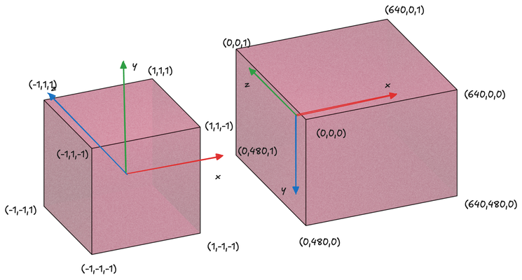
1. Conversion to Clip Space: The GPU transforms NDC to clip space coordinates using the formula (\frac{x_{ndc}}{w_{ndc}},\frac{y_{ndc}}{w_{ndc}},\frac{z_{ndc}}{w_{ndc}}). This step achieves the division by -z_{ndc} that we previously discussed.

2. Viewport Transformation: Next, clip coordinates are converted to viewport coordinates. This is where our viewport settings come into play. In viewport space:

• The x-axis points right

• The y-axis points down

• The coordinate range matches the viewport's width and height, as specified in the setViewport function

• The depth is mapped from [-1,1] to [minDepth, maxDepth], typically [0,1]

This image illustrates the mapping between NDC and viewport coordinates:

Mapping From NDC (Left) to the Viewport Coordinates (Right), With the Viewport Configured as (640,480,0,1)

It's important to note that after rasterization, fragment coordinates are in viewport coordinates. This can be counterintuitive, as we output clip coordinates from the vertex shader but receive viewport coordinates in the fragment shader, despite these variables sharing the same name. This distinction becomes crucial when implementing advanced effects like shadows in future chapters.

With this theoretical foundation, we can now implement a camera in WebGPU. Essentially, a camera is represented by two matrices:

1. A view matrix, determined by the camera's position and orientation

2. A projection matrix, based on the camera's aspect ratio and focal length

The glMatrix library provides convenient functions to generate these matrices efficiently. To apply these matrices to vertices, we use the same technique we've employed previously: passing the matrices as uniforms and performing matrix multiplication on vertex positions in the shader.

Let's examine the implementation details in the code:

@group(0) @binding(0)
var<uniform> transform: mat4x4<f32>;
@group(0) @binding(1)
var<uniform> projection: mat4x4<f32>;

@vertex
fn vs_main(
    @location(0) inPos: vec3<f32>,
    @location(1) inTexCoords: vec2<f32>
) -> VertexOutput {
    var out: VertexOutput;
    out.clip_position = projection * transform * vec4<f32>(inPos, 1.0);
    out.tex_coords = inTexCoords;
    return out;
}

The vertex shader undergoes minimal changes in this implementation. We've added a projection matrix alongside the existing transformation matrix. The transformation matrix repositions objects in front of the camera, converting coordinates from local space to view space. The projection matrix then applies the final transformation, projecting the view space to NDC. Both transformations are applied through simple matrix multiplications.

let transformationMatrix = glMatrix.mat4.lookAt(glMatrix.mat4.create(), 
glMatrix.vec3.fromValues(100, 100, 100), glMatrix.vec3.fromValues(0,0,0), glMatrix.vec3.fromValues(0.0, 0.0, 1.0));

let projectionMatrix = glMatrix.mat4.perspective(glMatrix.mat4.create(), 
1.4, 640.0 / 480.0, 0.1, 1000.0);

What's next is new to us: using glMatrix to generate both the transformation (view) matrix and the projection matrix. For simplicity, we assume the object is already in world coordinates, focusing on the conversion to view coordinates using the view matrix.

To generate the view matrix, we use the lookAt function, which takes three parameters:

• Position of the viewer

• Point the viewer is looking at

• Up vector of the camera

Note that while the up vector should ideally be orthogonal to the viewing direction, glMatrix will automatically adjust non-orthogonal vectors to ensure correct camera orientation.

For the projection matrix, we use the perspective function, which requires:

• Vertical field of view in radians (fovy), related to focal length

• Aspect ratio, typically viewport width/height

• Near bound of the frustum

• Far bound of the frustum

One of the advantages of using glMatrix is that it generates matrices as Float32Array objects, which can be directly loaded into GPU buffers:

let transformationMatrixUniformBuffer = createGPUBuffer(device, transformationMatrix, GPUBufferUsage.UNIFORM);

let projectionMatrixUniformBuffer = createGPUBuffer(device, projectionMatrix, GPUBufferUsage.UNIFORM);

let uniformBindGroupLayout = device.createBindGroupLayout({
    entries: [
        {
            binding: 0,
            visibility: GPUShaderStage.VERTEX,
            buffer: {}
        },
        {
            binding: 1,
            visibility: GPUShaderStage.VERTEX,
            buffer: {}
        },
        {
            binding: 2,
            visibility: GPUShaderStage.FRAGMENT,
            texture: {}
        },
        {
            binding: 3,
            visibility: GPUShaderStage.FRAGMENT,
            sampler: {}
        }
    ]
});

let uniformBindGroup = device.createBindGroup({
    layout: uniformBindGroupLayout,
    entries: [
        {
            binding: 0,
            resource: {
                buffer: transformationMatrixUniformBuffer
            }
        },
        {
            binding: 1,
            resource: {
                buffer: projectionMatrixUniformBuffer
            }
        },
        {
            binding: 2,
            resource: texture.createView()
        },
        {
            binding: 3,
            resource:
                sampler
        }
    ]
});

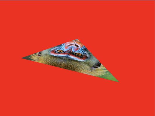
The uniform setup remains largely unchanged from previous examples. While the rendering result – a textured triangle viewed from an angle – might seem unexciting, this approach allows for incremental learning and provides a foundation for more complex implementations.

To challenge yourself and better understand the camera system, consider modifying this sample to create an animation where the camera rotates around the triangle. This exercise would involve:

• Updating the camera position in each frame

• Recalculating the view matrix

• Updating the uniform buffer with the new matrix

• Requesting a new frame for continuous animation

By implementing this animation, you'll gain practical experience in manipulating 3D camera systems and create a more dynamic and engaging visualization of the 3D space.

The Same Textured Triangle Is Viewed in an Angle