4.0 Prefix Sum
The focus of this chapter is compute shader, a new capability that is only available via WebGPU. with compute shader, we can harness the power of GPU to do general computation. AI inference, for instance, is an exciting example of what this can enable for the web.
The first tutorial will cover calculating the prefix sum (also known as scan), a fundamental component of numerous parallel algorithms. Subsequently, the second tutorial will leverage the prefix sum technique for sorting, another critical algorithmic operation. Finally, the third tutorial will showcase the integration of a compute shader for simulation alongside a rendering shader to craft an animated demonstration called "reaction diffusion".
Through these tutorials, we aim to illustrate the versatility and practicality of compute shaders, elucidating their significance in enhancing both computational and graphical capabilities within the realm of WebGPU.
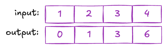
The prefix sum algorithm, when applied to an array of integers, generates a new array of the same length. Each element in this new array represents the summation of all elements preceding its position in the original array. For instance, considering the array [1, 2, 3], its prefix sum would be [0, 1, 3].
Prefix sums come in two variations: exclusive and inclusive. In exclusive prefix sums, each entry represents the summation of all elements before its position, excluding the element itself. On the other hand, inclusive prefix sums incorporate the value at the current position within the summation. In this tutorial, our focus will be on implementing the exclusive prefix sum algorithm.
Implementing prefix sum on a CPU using a for loop is straightforward. However, achieving efficiency in a parallel manner on the GPU presents a challenge. This challenge arises from the inherently sequential nature of the prefix sum operation. To calculate the value of an entry, it necessitates examining all its preceding entries, which inherently seems like a sequential operation. On the GPU, leveraging the massively parallel architecture for such an operation isn’t immediately intuitive due to the apparent dependency of each element's calculation on its predecessors.
Before working on the intricacies of the prefix sum algorithm, let's begin by understanding the general structure of setting up a compute shader and juxtapose it with a rendering shader. Initially examining the shader code, the differences may not seem extensive, but distinct nuances exist.
@binding(0) @group(0) var<storage, read> input :array<f32>;
@binding(1) @group(0) var<storage, read_write> output :array<f32>;
@binding(2) @group(0) var<storage, read_write> sums: array<f32>;
const n:u32 = 512;
var<workgroup> temp: array<f32,532>; //workgroup array must have a fixed size;
const bank_size:u32 = 32;
@compute @workgroup_size(256)
fn main(@builtin(global_invocation_id) GlobalInvocationID : vec3<u32>,
  @builtin(local_invocation_id) LocalInvocationID: vec3<u32>,
  @builtin(workgroup_id) WorkgroupID: vec3<u32>) {
      var thid:u32 = LocalInvocationID.x;
      var globalThid:u32 = GlobalInvocationID.x;
}
Firstly, our reliance shifts towards the storage buffer to input data, a facet less explored in rendering tasks. Utilizing a storage buffer over uniforms offers notable advantages. Notably, while uniforms aren't suitable for handling large data, storage buffers excel in this regard. While uniform buffer bindings are constrained to sizes up to 64KB (maxUniformBufferBindingSize), a storage buffer binding in WebGPU boasts a capacity of at least 128MB (maxStorageBufferBindingSize). Furthermore, storage buffers can be writable, proving particularly useful for reading back resulting data or preparing data for subsequent stages.
Additionally, our main function now bears the decoration @compute @workgroup_size(256). This introduces the concept of a "workgroup," which is unique to compute shaders. When invoking a compute shader, specifying the number of groups to invoke is a requirement. Each group comprises multiple threads, and the exact number of threads is defined by the @workgroup_size decoration. For instance, specifying 256 threads per group, the maximum allowed (maxComputeInvocationsPerWorkgroup), is exemplified here.
Despite sharing the term "threads", GPU threads differ from their CPU counterparts. In a CPU program, multiple threads can execute different programs concurrently. However, for GPU threads within the same workgroup, uniformity is mandatory—they must execute the same program.
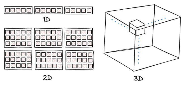
The thread count and group size can be specified in up to three dimensions for convenience. The choice of dimensionality hinges on the nature of the problem. the goal is to break down a large problem into smaller pieces, each for one thread to handle without interference with other threads. For instance, in image processing scenarios, employing 2D workgroups and threads might be most intuitive, allowing parallel computation for each pixel. Conversely, for tasks like the prefix sum, operating on a 1D array, utilizing 1D threads and groups proves to be the optimal choice.
The dimensionality of both groups and threads serves a purely convenience-driven purpose. Irrespective of the chosen dimensionality, their fundamental nature remains identical. In essence, a compute shader invocation follows a two-tier structure: the top tier comprises groups, and within each group reside individual threads. While the group count can be specified at runtime, the number of threads within each group remains static (hardcoded in shader).
A key distinction between compute shaders and rendering shaders is the absence of typical vertex attributes for inputs in compute shaders. However, compute shaders introduce specific built-ins that provide information to identify threads and groups. While compute shaders primarily rely on data input via storage buffers, these built-in IDs can effectively serve as indices to access data within these buffers.
Let's explore the concept of thread IDs and group IDs, supplied to a compute shader via built-in parameters of the main function. Each thread within a workgroup possesses an ID. If, for example, 256 threads are allocated within each group, the thread IDs range from 0 to 255. Importantly, launching multiple groups does not alter the range of thread IDs within each group; they continue to span from 0 to 255. These are referred to as the local_invocation_id. Additionally, we have the workgroup_id, which, in the scenario of launching three groups, spans from 0 to 2. To acquire a thread's ID among all threads in all launched workgroups, or the global ID, a simple formula applies: workgroup_id * workgroup_size + local_invocation_id. For convenience, WebGPU furnishes another built-in parameter called global_invocation_id.
It's crucial to note that both groups and threads can be organized in various dimensional configurations. Consequently, instead of a single number serving as an ID, an ID can manifest as a vector with x, y, and z components. How, then, do we compute a 2D or 3D global_invocation_id? We simply view groups and threads as matrices. Each group represents an entry within this matrix, while its threads form another matrix within that group.
Now that we've introduced the concept of workgroups, let's explore a new allocation type: var
The key aspect to note is that a workgroup buffer is confined to a specific group, restricting access for threads outside their respective groups. Usually, a workgroup buffer serves as a swift, localized storage solution—primarily designed for temporary data storage.
let pass1UniformBindGroupLayout = device.createBindGroupLayout({
    entries: [
        {
            binding: 0,
            visibility: GPUShaderStage.COMPUTE,
            buffer: { type: 'read-only-storage' }
        },
        {
            binding: 1,
            visibility: GPUShaderStage.COMPUTE,
            buffer: { type: "storage" }
        },
        {
            binding: 2,
            visibility: GPUShaderStage.COMPUTE,
            buffer: { type: "storage" }
        }
    ]
});
Let's explore setting up a compute shader in JavaScript. The initial step involves configuring the bind group layouts. Given the frequent use of storage buffers in compute shaders, when setting up bind group layouts for storage buffers, it's crucial to designate the buffer type as the storage type—specifically 'storage' for read and write operations and 'read-only-storage' for read-only access. Additionally, for buffer visibility, the setting now shifts to GPUShaderStage.COMPUTE.
Using storage buffers introduces a caveat, especially with certain data types like 'array
Consider 'array
It's crucial to note that the memory alignment requirement applies solely to the host-side memory preparation. Within the shader code, this additional padding remains transparent to the programmer, such that an 'array
const pass1PipelineLayoutDesc = { bindGroupLayouts: [pass1UniformBindGroupLayout] };
const pass1Layout = device.createPipelineLayout(pass1PipelineLayoutDesc);
const pass1ComputePipeline = device.createComputePipeline({
    layout: pass1Layout,
    compute: {
        module: pass1ShaderModule,
        entryPoint: 'main',
    },
});
const passEncoder = commandEncoder.beginComputePass(
    computePassDescriptor
);
passEncoder.setPipeline(pass1ComputePipeline);
passEncoder.setBindGroup(0, pass1UniformBindGroup);
passEncoder.dispatchWorkgroups(chunkCount);
passEncoder.end();
commandEncoder.copyBufferToBuffer(outputArrayBuffer, 0,
    readOutputArrayBuffer, 0, arraySize * 4);
commandEncoder.copyBufferToBuffer(outputSumArrayBuffer, 0,
    readSumArrayBuffer, 0, sumSize * 4);

device.queue.submit([commandEncoder.finish()]);
await device.queue.onSubmittedWorkDone();

await readOutputArrayBuffer.mapAsync(GPUMapMode.READ, 0, arraySize * 4);

const d = new Float32Array(readOutputArrayBuffer.getMappedRange());
Following that, configuring the compute pipeline bears resemblance to previous procedures. The notable difference lies in calling device.createComputePipeline and specifying a compute entry within its input. This entry delineates the entry point and the associated shader module for the compute pipeline.
The final step involves invoking the compute shader. Firstly, we initiate a compute pass by calling commandEncoder.beginComputePass. Once the compute pass is initiated, we set the pipeline and bind group as we did previously. However, instead of using functions like draw or drawIndexed, we utilize dispatchWorkgroups, specifying the desired group count. For instance, dispatchWorkgroups(2) launches 2 groups. It's important to remember that each group encompasses multiple threads. For example, configuring a group with 256 threads and launching 2 groups means deploying a total of 512 threads.
The group stands as the minimal unit for launching a compute shader. But what if the required number of threads isn't a multiple of 256? For instance, needing 600 threads would still entail launching 2 groups, resulting in extra threads. In the compute shader, it's crucial to inspect the global_invocation_id to identify these surplus threads, effectively managing them by assigning no operations ('doing nothing').
Having discussed how to configure a program involving compute shaders, let's now examine the prefix sum algorithm. Writing a naive prefix sum implementation isn't challenging — assigning each thread the task of computing the summation of all elements up to its global_invocation_id seems straightforward. However, this approach leads to redundant calculations, compromising efficiency.
An optimal parallel algorithm strives for 'work efficiency,' ensuring it doesn't perform excess work compared to a serialized version. Yet, if each thread is tasked with incorporating the summation computed by its preceding thread, it essentially necessitates every thread to wait for its predecessors to conclude their calculations. This sequentializes the entire process, negating the parallel benefits we seek to leverage.
Now, let's dive into our work-efficient parallel prefix sum. I'll begin by illustrating the concept using a tree structure. It's worth noting that I refer to this as an illustration, because in the actual code, we don't explicitly create a tree data structure. Constructing complex data structures involving pointers is challenging within shader code. Instead, the algorithm cleverly sidesteps this by exclusively using arrays. Yet, to grasp the underlying concept, envisioning a tree proves helpful.
The fundamental principle behind converting serialized algorithms into parallel ones involves breaking down the problem into smaller segments. Each thread then handles one of these segments, aggregating the results to form a smaller-sized problem. This process iterates until arriving at the final global result. Alternatively, another approach involves starting with a small problem and generating more results to create a larger set of independent problems. Parallel threads are then assigned to solve these, generating an even larger set of independent problems. Our prefix sum algorithm adeptly harnesses both of these techniques.
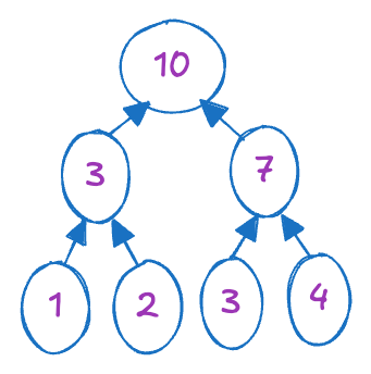
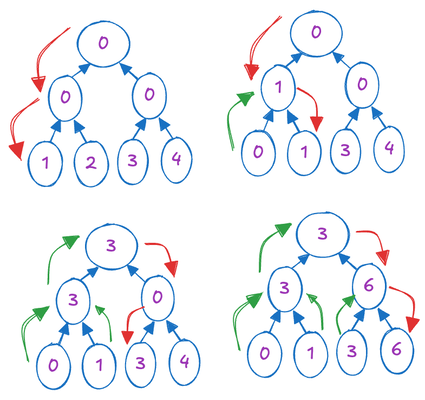
The algorithm's initial step involves a bottom-up process, constructing a binary tree where each node's value represents the summation of its subtrees. This aligns with the first approach mentioned earlier, where we commence by dividing the input array of size n into n/2 two-element arrays, aiming to compute the summation of each pair independently. This independent computation generates n/2 new values, effectively halving the problem size. This iterative process continues until reaching a single sum, representing the summation of all elements within the input array.
To demonstrate this process with a concrete example, consider an input array [1,2,3,4]. Initially, we divide this array into two two-element arrays: [1,2] and [3,4]. Simultaneously, we compute their summations in parallel, resulting in a new smaller array [3,7]. Continuing this process once more, we arrive at the final answer: 10.
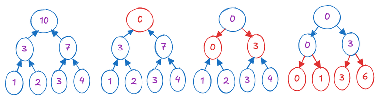
Having established the binary tree, the second step involves a top-down approach, moving from the root to the leaf nodes. We initialize the root node with zero. Then, progressing from the root towards the leaves, we apply the following operations in a layered manner: Each node computes the summation of its own value and its left child's value, assigning this result to the right child. Subsequently, the left child's value is updated with the current node's value. This process can be demonstrated using the illustration below.
Understanding the intuition behind this process might pose a challenge. Personally, I perceive it as a depth-first traversal of the binary tree, where, before visiting each leaf node, we've computed its prefix sum. The process described above primarily serves as an optimization for a straightforward and efficient GPU implementation, as Implementing an actual binary tree and performing tree traversal on the GPU presents significant challenges due to complexities involved.
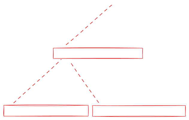
Let me explain the depth-first traversal approach using this illustration:
The initial array represents the leaf nodes. We traverse the tree in depth-first order, maintaining a temporary buffer to keep track of the current prefix sum. When we visit a leaf node, we replace its value with the current prefix sum and add the node's original value to the prefix sum. This process continues until all leaf nodes have been visited.
This method is analogous to the GPU implementation. Each node computes the summation of its own value and its left child's value, assigning this result to the right child, effectively passing the current prefix sum to the right child (Similar to the role of the temporary buffer in the above approach).
What we've described can be executed within a single group. Considering the largest thread size for a single group as 256 and a thread's ability to calculate the summation of two values enables us to process an array as large as 512 within a single group. However, when the input array surpasses 512 elements, we partition it into multiple 512-sized chunks, padding extra entries with zeros if needed. Multiple groups are then assigned to independently conduct the group-wise prefix sum in one pass, writing the total summation of each group into an intermediary output array.
In a subsequent pass, we perform another prefix sum of this intermediary output, assuming that the number of sums from the first step won't exceed 512. This assumption restricts the largest input array size to 512^2. To handle even larger arrays, we can continue this hierarchical scheme multiple times.
I'd like to clarify what I mean by a 'pass.' In our implementation, a pass typically represents a batch of execution through a dispatchWorkgroups function call. The groups launched in a single pass should not have interdependencies.
Why can't we treat multiple passes, such as two passes, as a single pass? The answer lies in the synchronization of groups. To utilize the results derived by a group and use it in a second pass, groups in the second pass must wait until all groups in the first pass have completed their calculations. However, there is no mechanism for groups to synchronize with each other; only threads within the same group have this capability, which we'll discuss shortly.
Ensuring all groups finish their work in the initial process requires enclosing it within a dedicated pass. By the completion of this pass, we can be certain that all groups have concluded their tasks. Subsequently, we proceed with the second pass.
After deriving the group prefix sum in the second pass, we initiate the third pass. Each group aggregates its local prefix sums with the group prefix sums before it.
Let's examine the actual code for pass 1:
@binding(0) @group(0) var<storage, read> input :array<f32>;
@binding(1) @group(0) var<storage, read_write> output :array<f32>;
@binding(2) @group(0) var<storage, read_write> sums: array<f32>;
const n:u32 = 512;
var<workgroup> temp: array<f32,532>; //workgroup array must have a fixed size;
Initially, we set up the input and output arrays. The output array saves the intermediate output by this group during the first pass, while the 'sums' houses the sums derived by all groups. 'n' represents the maximum array size this group can process.
Additionally, we introduce 'temp' as a temporary buffer used for calculations. It's defined as a workgroup allocation, which means it's confined within each group without global accessibility by other groups. Leveraging workgroup allocations enhances performance, making it advisable to use them wherever feasible to maximize performance."
Moving on to the main function, it receives the IDs specific to this group:
@compute @workgroup_size(256)
fn main(@builtin(global_invocation_id) GlobalInvocationID : vec3<u32>,
  @builtin(local_invocation_id) LocalInvocationID: vec3<u32>,
  @builtin(workgroup_id) WorkgroupID: vec3<u32>) {
      var thid:u32 = LocalInvocationID.x;
      var globalThid:u32 = GlobalInvocationID.x;
      if (thid < (n>>1)){
          temp[bank_conflict_free_idx(2*thid)] = input[2*globalThid]; // load input into shared memory
          temp[bank_conflict_free_idx(2*thid+1)] = input[2*globalThid+1];
      }
}
The 'workgroup_size' is set to 256, the maximum thread size we can request. Different ID types serve distinct purposes, and here, 'thid' represents the local thread ID, ranging from 0 to 255. On the other hand, 'globalThid' denotes the global ID.
Initially, the primary task involves loading input data into the 'temp' array. Each thread loads 2 consecutive values. Although it might seem unnecessary to check the boundary condition here since 'thid' is guaranteed to be smaller than (n >> 1) = 256, it's a good practice to implement boundary checks in shaders. Accessing indices out of range results in undefined behavior. Some implementations perform a clamp on accessing indices, leading to unexpected behavior, such as the last entry being consistently incorrect. In contrast, other implementations might treat out-of-range accesses as void operations. To mitigate these uncertainties or potential issues like incorrect values, implementing boundary checks before array access is advisable.
Next, we proceed with the bottom-up process:
workgroupBarrier();
var offset:u32 = 1;

for (var d:u32 = n>>1; d > 0; d >>= 1)
{
    if (thid < d)
    {
        var ai:u32 = offset*(2*thid+1)-1;
        var bi:u32 = offset*(2*thid+2)-1;
        temp[bank_conflict_free_idx(bi)] += temp[bank_conflict_free_idx(ai)];
    }
    offset *= 2;

    workgroupBarrier();
}
In this process, we loop log(512) times to cover the log(512) levels. At each level, a single thread is assigned to execute one summation of two entries in place. The resulting sum is then written to the second entry. An 'offset' variable indicates the interval between two entries at each level. Initially set to 1, this interval doubles as we halve the size of the problem in each layer.
An essential function to comprehend is workgroupBarrier(). This invokes a memory barrier that halts all threads at a specific point. Termed a workgroup barrier, it ensures that all previous writes to workgroup allocations (such as the temporary buffer) have completed before proceeding with reads. This precautionary step mitigates issues like read-before-write bugs.
Distinct from workgroup barriers, there are other memory barriers, such as storage barriers. While a storage buffer can be accessed by multiple groups (unlike a workgroup buffer), a storage barrier lacks the capability to synchronize these groups. For group synchronization, we rely on passes.
To conceptualize barriers, consider the analogy of a semaphore, a synchronization tool often studied in computer science courses. Though semaphores may not directly relate to GPU memory barriers, they aid in forming a mental model for understanding barriers.
Semaphores are employed to manage limited resources, analogous to a parking lot with finite spaces. A semaphore includes a counter indicating available resources. Upon resource utilization, a semaphore acquire operation decreases the counter. When the counter hits zero, signifying resource exhaustion, a thread attempting semaphore acquire halts until other threads execute semaphore release to increment the counter.
Similarly, envisioning a barrier, it also operates around a counter initialized to zero. When a thread triggers the barrier function, it effectively increments the counter. The barrier function only unblocks threads when the counter equals the total number of threads.
An essential aspect to bear in mind when dealing with synchronization-related operations is the crucial uniformity requirement. As specified in the spec: 'A collective operation necessitates coordination among concurrently running invocations on the GPU.' For an operation to execute correctly and consistently across different invocations, it must occur concurrently, adhering to uniform control flow. Collective operations encompass more than just barriers; they also encompass texture sampling functions. They too have the uniformity requirement, as we'll explain in subsequent chapters.
Conversely, collective operation in non-uniform control flow leads to incorrect behavior. This occurs when only a subset of invocations executes the operation or when they execute it non-concurrently due to non-uniform control flow. Such control flow arise from control flow statements relying on non-uniform values.
In simpler terms, regardless of the inputs received by shader code, a collective operation must be executed uniformly by all threads. For instance, the code snippet below is invalid and won't compile because only threads with an ID < 3 trigger workgroupBarrier(), while others won't. This conditional execution based on thread inputs violates uniformity as the operation must be executed by all threads irrespective of their inputs.
if (LocalInvocationID.x < 3) {
    workgroupBarrier();
}
Our conceptualization of a barrier with an internal thread counter makes it clear why non-uniform execution can cause issues. If only a subset of threads executes the barrier, the internal counter won't reach the total thread count, leading to indefinite blocking of threads that call it. Fortunately, this isn't a runtime scenario we'd encounter; the compiler will catch synchronization functions that violate the uniformity rule.
if (thid == 0)
{
    sums[WorkgroupID.x] = temp[bank_conflict_free_idx(n - 1)];
    temp[bank_conflict_free_idx(n - 1)] = 0;
} // clear the last element
workgroupBarrier();
The following code segments involve dumping the sum to the 'sum' array and resetting the sum in the 'temp' array to zero, priming it for the top-down process. As this operation is needed only once for the entire group, we designate the thread with ID zero to handle it.
The final step entails the top-down process and final output writing:
for (var d:u32 = 1; d < n; d *= 2) // traverse down tree & build scan
{
    offset >>= 1;
    if (thid < d)
    {
        var ai:u32 = offset*(2*thid+1)-1;
        var bi:u32 = offset*(2*thid+2)-1;
        var t:f32 = temp[bank_conflict_free_idx(ai)];
        temp[bank_conflict_free_idx(ai)] = temp[bank_conflict_free_idx(bi)];
        temp[bank_conflict_free_idx(bi)] += t;
    }
    workgroupBarrier();
}

if (thid < (n>>1)){
    output[2*globalThid] = temp[bank_conflict_free_idx(2*thid)];
    output[2*globalThid+1] = temp[bank_conflict_free_idx(2*thid+1)];
}
This concludes the first pass. By the end of this phase, we generate an output array containing the prefix sums of all groups, along with a sum array containing the total sum of all groups.
The second pass, akin to the first, is simpler as it only computes the prefix sum of sums without outputting the total sum. Details of this stage have been omitted.
The third pass is a straightforward process of augmenting each group's prefix sum with the sum of all preceding groups' sums.
var thid:u32 = LocalInvocationID.x;
var globalThid:u32 = GlobalInvocationID.x;
if (thid < (n>>1)){
  output[2*globalThid]= output[2*globalThid] + sums[WorkgroupID.x]; // load input into shared memory
  output[2*globalThid+1] = output[2*globalThid+1] + sums[WorkgroupID.x];
}
Now, let's explore the JavaScript code to observe the invocation of these three passes. For both the first and third passes, we initiate a number of workgroups equal to chunkCount. Calculating chunkCount involves utilizing the expression Math.ceil(arraySize / 512);, ensuring it represents the smallest multiple of 512 capable of accommodating the problem size. Conversely, the second pass is executed with just a single group, consequently limiting the maximum problem size to 512^2.
passEncoder.setPipeline(pass1ComputePipeline);
passEncoder.setBindGroup(0, pass1UniformBindGroup);
passEncoder.dispatchWorkgroups(chunkCount);
passEncoder.end();
const pass2Encoder = commandEncoder.beginComputePass(computePassDescriptor);
pass2Encoder.setPipeline(pass2ComputePipeline);
pass2Encoder.setBindGroup(0, pass2UniformBindGroup);
pass2Encoder.dispatchWorkgroups(1);
pass2Encoder.end();

const pass3Encoder = commandEncoder.beginComputePass(computePassDescriptor);
pass3Encoder.setPipeline(pass3ComputePipeline);
pass3Encoder.setBindGroup(0, pass3UniformBindGroup);
pass3Encoder.dispatchWorkgroups(chunkCount);
pass3Encoder.end();
Before concluding this tutorial, it's important to address benchmarking for our GPU code. Since GPU code executes on a separate device, assessing GPU execution solely on the CPU side may not yield accurate results. Fortunately, WebGPU offers an extension that facilitates performance measurement.
The extension is called 'timestamp-query,' an experimental feature in Chrome that requires special enabling via the --enable-dawn-features=allow_unsafe_apis command line option:
/Applications/Google\ Chrome.app/Contents/MacOS/Google\ Chrome --enable-dawn-features=allow_unsafe_apisTo request this feature from the adapter, follow this JavaScript snippet:
const adapter = await navigator.gpu.requestAdapter();

const hasTimestampQuery = adapter.features.has('timestamp-query');

let device = await adapter.requestDevice({
    requiredFeatures: hasTimestampQuery ? ["timestamp-query"] : [],
});
For better cross-browser compatibility, consider safeguarding benchmark-related code within the hasTimestampQuery condition. This ensures that in cases where the browser flag isn't provided or the extension isn't supported, it won't cause any runtime errors.
The 'timestamp-query' functionality operates by allowing you to request a temporary storage termed a query set. During command buffer encoding, you can instruct the GPU to record the current timestamp into this query set. Once the timing process is complete, you can transfer the query set to a buffer. After the command buffer finishes, the timestamps can be accessed by copying the buffer to the host. As the timing occurs entirely on the GPU, it ensures accuracy.
const capacity = 3;//Max number of timestamps we can store
const querySet = hasTimestampQuery ? device.createQuerySet({
    type: "timestamp",
    count: capacity,
}) : null;

const queryBuffer = hasTimestampQuery ? device.createBuffer({
    size: 8 * capacity,
    usage: GPUBufferUsage.QUERY_RESOLVE
        | GPUBufferUsage.STORAGE
        | GPUBufferUsage.COPY_SRC
        | GPUBufferUsage.COPY_DST,
}) : null;
In this example, the 'capacity' is set to 3, allowing the storage of up to 3 timestamps in the buffer. Given that each timestamp is a 64-bit integer, the 'queryBuffer' size is requested to be 8 times the 'capacity' to accommodate these integers.
Here is how we perform timing:
if (hasTimestampQuery) {
    commandEncoder.writeTimestamp(querySet, 0);// Initial timestamp
}

... // perform the compute passes

if (hasTimestampQuery) {
    commandEncoder.writeTimestamp(querySet, 1);// Second timestamp
    commandEncoder.resolveQuerySet(
        querySet,
        0,// index of first query to resolve
        capacity,//number of queries to resolve
        queryBuffer,
    0);// destination offset
}
When we wish to extract the data from the query set, the resolveQuerySet function is called to achieve this. After the command buffer completes its execution, we proceed to retrieve the buffer's data, following a similar process to what we previously employed for handling different buffer types:
if (hasTimestampQuery) {
    const gpuReadBuffer = device.createBuffer({ size: queryBuffer.size, usage: GPUBufferUsage.COPY_DST | GPUBufferUsage.MAP_READ });
    const copyEncoder = device.createCommandEncoder();
    copyEncoder.copyBufferToBuffer(queryBuffer, 0, gpuReadBuffer, 0, queryBuffer.size);
    const copyCommands = copyEncoder.finish();
    device.queue.submit([copyCommands]);
    await gpuReadBuffer.mapAsync(GPUMapMode.READ);
    let result = new BigInt64Array(gpuReadBuffer.getMappedRange());
    console.log("run time: ", (result[1] - result[0]));
    gpuReadBuffer.unmap();
    gpuReadBuffer.destroy();
}
Notice that due to the timestamp being of type int64, we employ buffer mapping to a BigInt64Array, allowing us to measure time in nanoseconds.
Another crucial consideration is bank conflict within the workgroup memory. Unlike other memory types, workgroup memory is organized into banks. If multiple threads attempt to access the same bank simultaneously, their execution becomes serialized. In other words, one thread must wait for another to finish accessing the bank before it can proceed. This phenomenon is known as bank conflict, a critical aspect that GPU programmers need to optimize for. It's important to note that memory organization is hardware-dependent.
The information presented here is based on NVIDIA's documentation and is commonly treated as the default configuration. However, when dealing with Apple's silicon, detailed information regarding memory organization may be lacking. In such cases, optimization strategies need to be derived from benchmarks and experiments rather than relying on explicit documentation.
For most hardware, continuous workgroup allocation advances one bank every 32 bits. As an example, if we have an array