1.8 Utilizing Transformation Matrices

In this tutorial, we'll revisit our previous shader example to achieve the same result—an offset triangle. However, this time, we'll employ a transformation matrix instead of a simple offset vector. By multiplying our vertex positions with this transformation matrix, we'll produce the same outcome. The key takeaway is that adding an offset vector is equivalent to applying a transformation matrix.

Transformation matrices offer a more versatile way to represent transformations. In practice, we rarely limit ourselves to applying offsets alone. These matrices can handle not just offsetting but also scaling, rotation, and projection. Indeed, transformation matrices are the most generic way of manipulating vertex position. For aspiring graphics developers, a thorough understanding of transformation matrices is crucial—it's an unavoidable aspect of graphics programming.

If you're new to graphics development, this concept might seem challenging. Let's take a step-by-step approach to make sense of it. We'll start with 2D examples and concrete scenarios. In this tutorial, our focus will be on scaling, translation, and rotation. We'll explore the projection matrix in the next chapter.

Scaling

Scaling is the simplest transformation to understand. Imagine we have a 2D vector (x,y). If we want to scale this vector by a factor of 3, the stretched vector becomes (3x,3y). We can apply different multipliers to x and y; for instance, using (3,4) would result in (3x,4y). The equation for 2D scaling is straightforward:

\begin{aligned} x^\prime &= 3 \times x \\ y^\prime &= 4 \times y \\ \end{aligned}

We can rewrite this calculation in a less intuitive matrix multiplication form. By the end of this tutorial, you should appreciate why matrices are the preferred way of representing transformations in computer graphics.

\begin{pmatrix} 3 & 0 \\ 0 & 4 \end{pmatrix} \times \begin{pmatrix} x \\ y \end{pmatrix} = \begin{pmatrix} 3x \\ 4y \end{pmatrix}

This calculation extends easily to 3D space:

\begin{pmatrix} 3 & 0 & 0 \\ 0 & 4 & 0 \\ 0 & 0 & 5 \end{pmatrix} \times \begin{pmatrix} x \\ y \\ z \end{pmatrix} = \begin{pmatrix} 3x \\ 4y \\ 5z \end{pmatrix}

Translation

Translation is slightly more complex. Let's start with 2D again. If we want to offset a 2D point (x,y) by (3,4), we calculate the new point as:

\begin{aligned} x^\prime &= 3 + x \\ y^\prime &= 4 + y \\ \end{aligned}

Rewriting this as a matrix multiplication isn't immediately obvious. We can attempt it:

\begin{pmatrix} 1 & \frac{3}{y} \\ \frac{4}{x} & 1 \end{pmatrix} \times \begin{pmatrix} x \\ y \end{pmatrix} = \begin{pmatrix} x + 3 \\ 4 + y \end{pmatrix}

While this works, it's not ideal because the translation matrix is tied not only to the desired offset but also to the vector (x,y). Without knowing the vector, we can't derive the translation matrix. This is undesirable in graphics applications, where we want to define a transformation matrix once and apply it to any vertex, creating the same transformation regardless of the vertex's actual position.

We can employ a clever trick to make the translation matrix depend only on the offset:

\begin{pmatrix} 1 & 0 & 3 \\ 0 & 1 & 4 \\ 0 & 0 & 1 \end{pmatrix} \times \begin{pmatrix} x \\ y \\ 1 \end{pmatrix} = \begin{pmatrix} x + 3 \\ y + 4 \\ 1 \end{pmatrix}

Here, we're expanding the matrix to 3x3, with the offset defined in the last column. We also extend the point location to a 3x1 vector so it can still multiply with the matrix. Now the translation matrix relates only to the offset, and multiplying it with the vector yields (x+3, y+4, 1), where the first two elements represent the offset 2D point.

This approach seems to add extra data and calculation, but it creates a matrix with our desired properties. We can also modify the 2D scaling matrix by extending it to 3x3, giving it the same form as the translation matrix.

Extending this to 3D is straightforward; we simply use a 4x4 matrix:

\begin{pmatrix} 1 & 0 & 0 & 3 \\ 0 & 1 & 0 & 4 \\ 0 & 0 & 1 & 5 \\ 0 & 0 & 0 & 1 \end{pmatrix} \times \begin{pmatrix} x \\ y \\ z \\ 1 \end{pmatrix} = \begin{pmatrix} x + 3 \\ y + 4 \\ z + 5 \\ 1 \end{pmatrix}

Rotation

Rotation is the most challenging transformation to conceptualize. Imagine we have a 2D vector (x,y) that we want to rotate by an angle \theta. Let's first manually calculate the rotation, assuming (x,y) is a unit vector. We'll then consider how to rotate a vector of any length.

Rotate a 2D Vector (X,Y) by an Angle Θ

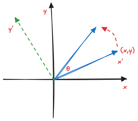
To rotate the vector by \theta, we can construct a new coordinate system where (x,y) is the x^\prime axis and (-y, x) is the y^\prime axis. In this new system, the rotated vector and the x^\prime axis form an angle \theta.

The rotated vector's position in the new coordinate system is (cos(\theta)x^\prime, sin(\theta)y^\prime). Substituting x^\prime with (x,y) and y^\prime with (-y,x), we get the new vector in the original coordinate system: (cos(\theta)x-sin(\theta)y, cos(\theta)y+sin(\theta)x).

We can rewrite this calculation as a matrix multiplication:

\begin{pmatrix} cos(\theta) & -sin(\theta) \\ sin(\theta) & cos(\theta) \end{pmatrix} \times \begin{pmatrix} x \\ y \end{pmatrix} = \begin{pmatrix} cos(\theta)x - sin(\theta)y\\ sin(\theta)x + cos(\theta)y \end{pmatrix}

For non-unit vectors, we can normalize by the length l = \sqrt{x^2+y^2}, rotate, and then scale back. You'll find that the rotation matrix is independent of the vector size and only relates to the rotation angle.

Our goal in rewriting these calculations as matrix multiplications is to unify the form of the calculation. Regardless of the transformation, it can be achieved through matrix multiplication. This allows us to chain multiple transformations easily by multiplying several matrices with a vector. Each matrix represents a transformation, and we can merge a series of transformation matrices into a single matrix through multiplication. This property is crucial for deriving the rotation matrix for 3D space.

Having derived the rotation matrix for the xy plane, we can easily extend this to the xz and yz planes. Any complex rotation in 3D can be decomposed into a three-step rotation in each plane. Assuming angles \theta_{xy}, \theta_{xz}, and \theta_{yz}, the 3D rotation matrix would be:

\begin{pmatrix} 1 & 0 & 0 \\ 0 & cos(\theta_{yz}) & -sin(\theta_{yz}) \\ 0 & sin(\theta_{yz}) & cos(\theta_{yz}) \end{pmatrix} \times \begin{pmatrix} cos(\theta_{xz}) & 0 & -sin(\theta_{xz}) \\ 0 & 1 & 0 \\ sin(\theta_{xz}) & 0 & cos(\theta_{xz}) \end{pmatrix} \times \begin{pmatrix} cos(\theta_{xy}) & -sin(\theta_{xy}) & 0 \\ sin(\theta_{xy}) & cos(\theta_{xy}) & 0 \\ 0 & 0 & 1 \end{pmatrix}

With these three types of transformation matrices, you can perform almost all transformations except for projection. Perspective projection, for example, makes distant objects appear smaller than closer ones, matching our real-life experience. This deformation can't be achieved solely through rotation, translation, and scaling. We'll explore projection in the next chapter as it's crucial for implementing cameras in 3D graphics.

Homogeneous Coordinates

If we only concerned ourselves with scaling and rotation, 3x3 matrices would suffice. However, to include translation, we need to extend the matrices to 4x4 and vectors to 4x1. Recall that in our previous shader code, the vertex shader's position output was always a vec4<f32>, with the fourth element set to 1.0. Now you understand why. These 4D vectors are called homogeneous coordinates. The fourth element isn't always 1; it's 1 for points and 0 for vectors. This distinction is important because vectors, which always start from the origin, can be scaled or rotated but not translated. Setting the fourth element to zero ensures that vectors remain unaffected by translation in any transformation matrix.

When the fourth element is not 1 or 0, the value is treated as a scaling factor. The actual position of the point can be obtain by (\frac{x}{w},\frac{y}{w},\frac{z}{w}).

Now that we've introduced transformation matrix theory, let's explore its practical implementation. In addition to transformation matrices, I'll introduce you to a valuable third-party library called glMatrix. While manually creating transformation matrices for 2D points isn't too challenging, it becomes quite tedious for 3D points. This is where glMatrix proves invaluable; it can generate transformation matrices and handle various vector and matrix-related calculations extensively used in computer graphics. We'll rely on this library throughout our journey in this book.

@group(0) @binding(0)
var<uniform> transform: mat4x4<f32>;

@vertex
fn vs_main(
    @location(0) inPos: vec3<f32>,
    @location(1) inTexCoords: vec2<f32>
) -> VertexOutput {
    var out: VertexOutput;
    out.clip_position = transform * vec4<f32>(inPos, 1.0);
    out.tex_coords = inTexCoords;
    return out;
}

We've updated our shader code, replacing the vec3 uniform called offset with a new uniform named transform of type mat4x4<f32>. This change alters how we calculate the clip position. In the previous version, we added the inPos variable to the offset vector to determine the final position. Now, we achieve this by directly multiplying the inPos vector with the transformation matrix.

let translateMatrix = glMatrix.mat4.fromTranslation(glMatrix.mat4.create(), glMatrix.vec3.fromValues(-0.5, -0.5, 0.0));

let uniformBuffer = createGPUBuffer(device, translateMatrix, GPUBufferUsage.UNIFORM);

Let's examine the setup of the uniform buffer. While most of it remains similar, the key difference lies in how we generate the transformation matrix.

Since our transformation involves only translation, we utilize the glMatrix library's fromTranslation helper function. This library provides a comprehensive set of vectors and matrices utilities of various dimensions, such as vec2 and mat4. For each type, it offers numerous functions for performing algebraic calculations or constructing values tailored to our needs. For instance, fromTranslation creates a new matrix based on an offset vector, while fromRotation generates a matrix defining a rotation. Additionally, fromRotationTranslation can produce a matrix combining both rotation and translation.

If you're accustomed to programming languages other than JavaScript, you might find glMatrix's syntax somewhat verbose. This verbosity primarily stems from JavaScript's lack of operator overloading. However, once you become familiar with glMatrix, this extra verbosity becomes less of an issue.

For those interested in the generated translation matrix, you can print its values and manually verify that multiplying it with the vertices indeed achieves the desired offset.

The rest of the code remains largely unchanged. We create a uniform buffer and copy the internal values of the translation matrix (16 floats) into this buffer using our convenient helper function createGPUBuffer.

Upon running the code, you'll observe the same offset triangle. Challenge yourself by deriving different translation matrices by altering the input of the fromTranslation function. You can also experiment with the fromRotationTranslation function to see if you can rotate the triangle as well.

While the sample code in this chapter is relatively basic, the key focus lies on understanding the transformation matrix. In subsequent chapters, you'll find this concept being applied extensively across various scenarios.